- IP (Internet Protocol) https://www.rfc-editor.org/rfc/rfc791.txt
- UDP (User Datagram Protocol) https://www.rfc-editor.org/rfc/rfc768.txt
- TCP (Transmission Control Protocol) https://www.rfc-editor.org/rfc/rfc793.txt
- Official Arpa-internet Protocols https://www.rfc-editor.org/rfc/rfc991.txt
- Address Allocation for Private Internets https://www.rfc-editor.org/rfc/rfc1918.txt
- NAT - The IP Network Address Translator https://www.rfc-editor.org/rfc/rfc1631.txt
- Traditional NAT - Traditional IP Network Address Translator https://www.rfc-editor.org/rfc/rfc3022.txt
- STUN - Simple Traversal of User Datagram Protocol (UDP) https://www.rfc-editor.org/rfc/rfc3489.txt
- NAT Behavioral Requirements for Unicast UDP https://www.rfc-editor.org/rfc/rfc4787.txt
- NAT Behavioral Requirements for TCP https://www.rfc-editor.org/rfc/rfc5382.txt
- NAT Behavioral Requirements for ICMP https://www.rfc-editor.org/rfc/rfc5508.txt
互联网(Internet)起源于美国,最初由战争驱动技术发展。Internet 一词由 Interconnected networks 组合而成。
美国国防高级研究计划局(Defense Advanced Research Projects Agency),简称DARPA,是美国国防部属下的一个行政机构,负责研发用于军事用途的高新科技。成立于1958年,当时的名称是“高等研究计划局”(Advanced Research Projects Agency,简称ARPA),1972年3月改名为DARPA,但在1993年2月改回原名ARPA,至1996年3月再次改名为DARPA。
RFC 991 Official Arpa-internet Protocols 文档包含了 ARPA 官方协议的说明,按三个层次分类:
- NETWORK LEVEL
- HOST LEVEL
- APPLICATION LEVEL
互联网通信基于 IP 协议,此协议需要使用一个网络地址,即 IP 地址,早期的使用的 IPv4 地址使用 4 个字节,总共有 4,294,967,296 个地址。这些地址看似好多,但是全球都在使用,人均也分不到一个, 并且组建网络本身的设备也需要使用 IP 地址,还有些保留专用的地址,所以 IPv4 地址根本不够用。 最新的 IPv6 地址使用 128 bits (16 bytes),网络号、主机号各占 64 bits 8 个字节。并且, 网络号通常由 media access control (MAC) 或其它网络接口标识构成。显示为 8 组十六进制符号, 每组两个字节,每个 x 代表 4 bits:xxxx:xxxx:xxxx:xxxx:xxxx:xxxx:xxxx:xxxx。 IPv6 地址支持压缩前导零的表示方法,每段连续的 0 也可以压缩为一个 0,多段的 0 值压缩为 :: 双冒号。注意的是:双冒号只能出现一次。
IP 地址包含网络号(Network number/ID)和主机号(Host number/ID),使用 32 bits 掩码来标记。 RFC 790/791 文档中将 32-bit 得 IP 地址根据不同网络号划分成三个类型:
Address Formats:

  High Order Bits   Format                           Class
  ---------------   -------------------------------  -----
        0            7 bits of net, 24 bits of host    A
        10          14 bits of net, 16 bits of host    B
        110         21 bits of net,  8 bits of host    C
        111         escape to extended addressing mode
A 类地址最高位为 0,使用 7-bit 表示网络号 network number,24-bit 表示本地主机地址,可以分配 128 个 A 类网络。
   0                 1                   2                   3
   0 1 2 3 4 5 6 7 8 9 0 1 2 3 4 5 6 7 8 9 0 1 2 3 4 5 6 7 8 9 0 1
  +-+-+-+-+-+-+-+-+-+-+-+-+-+-+-+-+-+-+-+-+-+-+-+-+-+-+-+-+-+-+-+-+
  |0|   NETWORK   |                Local Address                  |
  +-+-+-+-+-+-+-+-+-+-+-+-+-+-+-+-+-+-+-+-+-+-+-+-+-+-+-+-+-+-+-+-+

         Class A Address 0.0.0.0 ~ 127.255.255.255
B 类地址最高位为 10,使用 14-bit 表示网络号,16-bit 表示本地主机地址,可以分配 16,384 个 B 类网络。
   0                 1                   2                   3
   0 1 2 3 4 5 6 7 8 9 0 1 2 3 4 5 6 7 8 9 0 1 2 3 4 5 6 7 8 9 0 1
  +-+-+-+-+-+-+-+-+-+-+-+-+-+-+-+-+-+-+-+-+-+-+-+-+-+-+-+-+-+-+-+-+
  |1 0|           NETWORK         |          Local Address        |
  +-+-+-+-+-+-+-+-+-+-+-+-+-+-+-+-+-+-+-+-+-+-+-+-+-+-+-+-+-+-+-+-+

         Class B Address 128.0.0.0 ~ 191.255.255.255
C 类地址最高位为 110,使用 21-bit 表示网络号,8-bit 表示本地主机地址,可以分配 2,097,152 个 C 类网络。
   0                 1                   2                   3
   0 1 2 3 4 5 6 7 8 9 0 1 2 3 4 5 6 7 8 9 0 1 2 3 4 5 6 7 8 9 0 1
  +-+-+-+-+-+-+-+-+-+-+-+-+-+-+-+-+-+-+-+-+-+-+-+-+-+-+-+-+-+-+-+-+
  |1 1 0|                    NETWORK              | Local Address |
  +-+-+-+-+-+-+-+-+-+-+-+-+-+-+-+-+-+-+-+-+-+-+-+-+-+-+-+-+-+-+-+-+

         Class C Address 192.0.0.0 ~ 224.255.255.255
一些殊用途 IP:
-
回环地址(Loopback address)
-
网段地址 (Segment address)
-
广播地址(Broadcast address)
-
私有 IP 地址,在私有网络中使用的地址,不被公共互联网路由器转发。
RFC 1918 Address Allocation for Private Internets 文档简要地说明了保留的私用 IP 地址:
- Private Address Space
The Internet Assigned Numbers Authority (IANA) has reserved the following three blocks of the IP address space for private internets:
10.0.0.0 - 10.255.255.255 (10/8 prefix) 172.16.0.0 - 172.31.255.255 (172.16/12 prefix) 192.168.0.0 - 192.168.255.255 (192.168/16 prefix) -
0.0.0.0(未指定地址):表示不确定的目标或任意目标。可用作服务器绑定地址,表示监听所有可用的网络接口。
-
255.255.255.255(广播地址):用于向本地网络中的所有设备广播消息。
-
169.254.0.0 ~ 169.254.255.255:用于自动配置 IP 地址,当设备无法通过 DHCP 获取有效的 IP 地址时,会使用此地址范围进行自我配置。
-
224.0.0.0 ~ 239.255.255.255:用于多播(Multicast)通信,允许将数据同时发送到多个设备。
网络号为 127 的地址都是回环地址,计算机用于自我回路测试和通信,也就是指向当前主机,例如 127.0.0.1。
127.0.0.0 表示网段地址,不能用于通信,执行 ping 127.0.0.0 只能得到“一般故障”。
主机标识段 Host ID 比特位为 1 的 IP 地址为广播地址,广播的分组传送给 Host ID 涉及的所有计算机。 例如,IP 地址 10.1.1.0,对应掩码 255.0.0.0,其网段广播地址为 10.255.255.255。向此广播地址 发送数据包时,它将被分发给该网段(10.0.0.0)上的所有计算机。
单播(Unicast)、多播(Multicast)和广播(Broadcast)是三种通信形式:
-
单播:两个网络节点之间的通信,此时信息的接收和传递只在两个节点之间进行。最普遍的通信形式,例如,收发电子邮件、浏览网页时,当前主机必须与邮件服务器、Web服务器建立连接,此时使用的就是单播数据传输方式。通常使用“点对点通信”(Point to Point)代替“单播”,因为“单播”一般与“多播”和“广播”相对应使用。
-
多播:也称为“组播”,网上视频会议、网上视频点播特别适合采用多播方式,一台主机同时为多台客户机提供服务。IP 网络的多播用专用的地址段,即 224.0.0.0 ~ 239.255.255.255 之间的 IP 地址,它们属于 D 类 IP 地址。
-
广播:一台主机主动向多台主机发送消息,在网络中的应用较多。如客户机通过 DHCP 服务自动获得 IP 地址的过程就是广播形式,向网段中的所有主机请求 IP 申请消息,而收到消息的主机中如果有 DHCP 服务器,就会响应客户端请求。同单播、多播相比,广播几乎占用了子网内网络的所有带宽。当网络中充斥无法处理的广播消息,就会形成“广播风暴”,蠕虫病毒和 ARP 攻击是造成网络广播风暴最主要的原因。IP 网络使用专用的广播地址,其中 255.255.255.255 是通用的广播地址,这个 IP 地址代表同一子网内所有的 IP 地址。
广播域(Broadcast domain)是指接收同样广播消息的节点的集合。在该集合中的任何一个节点传输一个广播帧,则所有其他能收到这个帧的节点都被认为是该广播帧的一部分。广播帧是指目标 MAC 地址 48 bits 全部为 1 的数据帧。不仅仅是广播帧,多播帧(Multicast Frame)和目标不明的单播帧(Unknown Unicast Frame)也能在同一个广播域中畅行无阻。
冲突域(物理分段)是连接在同一导线上的所有工作站的集合,或者说是同一物理网段上所有节点的集合或以太网上竞争同一带宽的节点集合。这个域代表了冲突在其中发生并传播的区域,这个区域可以被认为是共享段。冲突域看作是 OSI 模型中第一层的概念,连接同一冲突域的设备有 Hub、Reperter,或者其他进行简单复制信号的设备。也就是说,Hub、Repeater 等设备连接的所有节点可以被认为是在同一个冲突域内,它们不会划分冲突域。而第二层设备(网桥,交换机)第三层设备(路由器)都可以划分冲突域的,当然也可以连接不同的冲突域。简单的说,可以将Repeater等看成是一根电缆,而将网桥等看成是一束电缆。
网络应用中使用模型概念:
| OSI 七层网络模型 | TCP/IP 模型 | 对应网络协议 |
|---|---|---|
| 应用层(Application) | 应用层 | HTTP、TFTP, FTP, NFS, WAIS、SMTP |
| 表示层(Presentation) | 应用层 | Telnet, Rlogin, SNMP, Gopher |
| 会话层(Session) | 应用层 | SMTP, DNS |
| 传输层(Transport) | 传输层 | TCP, UDP |
| 网络层(Network) | 网络层 | IP, ICMP, ARP, RARP, AKP, UUCP |
| 数据链路层(Data Link) | 数据链路层 | FDDI, Ethernet, Arpanet, PDN, SLIP, PPP |
| 物理层(Physical) | 硬件 | IEEE 802.1A, IEEE 802.2 ~ IEEE 802.11 |
网络应用开发需要理解 OSI 分层概念,特别是 Layer 2 ~ 4,它们与 TCP/IP 编程模型关系密切:
-
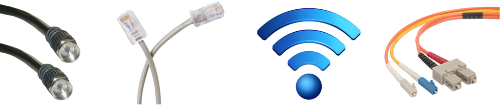
OSI Layer 1 – Physical
物理层对应的是网络的连接介质,通过电缆、光纤、中继器(Repeaters)、集线器(Hubs) 传输比特码,即 1、0 电脉冲信号(the 1’s and 0’s)。
中继器用于直接转发电脉冲信号,并且可以补偿信号在传输过程中的衰减。集线器相当于多口中继器,各个端口的信息互通。
-
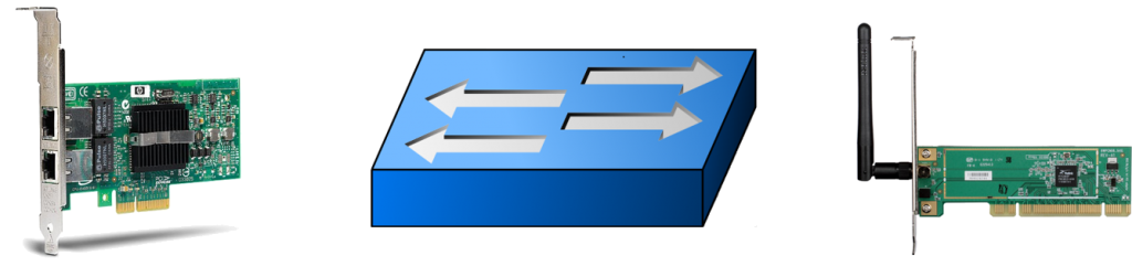
OSI Layer 2 – Data Link
数据链路层,Data Link layer,响应 OSI 物理层接口。实际上,数据链路负责在电缆、光纤上放置、接收 1、0 电脉冲信息(the 1’s and 0’s)。网卡(NIC - Network Interface Card)上插入的以太网电缆就是对应数据链路层的功能,比特脉冲信息通过电缆上传递,接收和发送。对于无线网卡(WIFI NIC),也以同样方式传递比特信号,只不过是无线电波替代了电缆上的电脉冲。
除了 NIC,交换机(Switch)也工作在数据链路层,交换机的主要职责是负责协调本网络的通信,包括:
- Learning 学习网络拓扑结构
- Flooding 流量控制
- Forwarding 数据转发
- Filtering 数据过滤
数据链路层收发的比特数据对应的是数据帧(Frame),此层寻址系统是物理地址(MAC - Media Access Control),使用 48 bits 共 6 个字节表示。MAC 地址在硬件厂商生产过程中就已经确定,有时也称为硬件地址,或者 Burned In Address (BIA)。
ipconfig -all; sleep 30总结:数据链路层通过 NIC 之间的电缆或无线信号收发数据帧,数据收发 hop to hop,每个 NIC 对应跃点(Hop)。
-
OSI Layer 3 – Network
网络层逻辑上使用 IP 协议地址来确实网络上的节点(端点,end),因此数据包的传输形式是 end to end。不同于固定(绑定)在硬件内的 MAC 地址,IP 是临时分配的地址。路由器作为网络连接中主要角色,其工作于网络层,协调网络之间的通信,这一点与交换机区别。因此,路由器对应着两个网络之间的一个边界。要与其它网络的设备通信,就必需经过路由器。

-
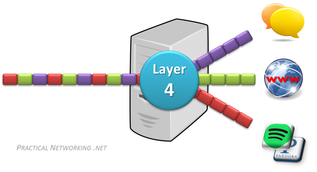
OSI Layer 4 – Transport
传输层对应的是网络流量,数据在计算机网卡 NIC - Network Interface Card 中以补码、反码(1’s and 0’s)形式表示。这些数据流可能是浏览器中看到的 Web 页面、Email 中阅读的内容、网络音乐播放器中的声音。为了区分这些网络流量,传输层就引入了 PORT,对应的是 TCP/UDP 协议中使用的端口,两协议各自使用 32 bits 数据表示端口,可以表达 65,536 个端口。TCP/UDP 端口是其一种网络传输标识符(Transport identifier),还有 ICMP query ID,也是。系统通过数据包中的 IP 地址(来源地址、目标地址)和 TCP/UDP 的端口组合来区分数据流属于什么应用程序。
总结来说,如果 Layer 2 对应 hop to hop 的数据传输,Layer 3 对应 end to end 的数据传输,那么 Layer 4 就对应 service to service 的数据传输。TCP/UDP 和 Port 是传输层的标志,也是网络应用开发人员主要的网络基础知识。
-
OSI Layer 5, 6, 7 - Session, Presentation, Application
会话层、表示层、应用层是 OSI 模型在数据呈送给最终用户前的最终阶段。对于一个纯粹的网络工程师而言,区别对待这三层的意义不大。反而使用 TCP/IP 模型更有意义,它们统一作为应用层看待,对应的就是应用程序中 socket 编程接口收发的数据。工程师们常用 L5-7 或 L5+ 或 L7 这样的简化形式表达。
理解以上 OSI Model 基础后,作为网络开发工程师,就需要对 Layer 2 ~ 4 有深刻的认识,即对应 IP、MAC/TCP、UDP/Port 三层内容。其中 Layer 2 ~ 3 又更贴近硬件层面,也更贴近计算机网络通信的核心,它们对应了计算机网络最重要的两个寻址系统:
- Layer 2 使用 MAC 地址,负责 hop to hop 的数据包收发;
- Layer 3 使用 IP 地址,负责 end to end 的数据包收发;
当计算机需要发送数据时,需要先将数据包装到 IP 包中,IP 包头部包含通信双端(end to end)的 IP 地址(Source IP 和 Destination IP)。然后再继续打包到 MAC 数据帧(Frame),其帧头部包含了通信双方(hop to hop)的 MAC 地址(Source MAC 和 Destination MAC)。
在网络传输过程中,IP 地址或者 MAC 地需要根据实际情况进行变更。数据的接收方,包含 MAC 地址的数据帧(Frame)头部会在路由上剥离,并按路由表记录的下一个 hop 的数据重新生成数据帧头部。当数据包到达最终的目标计算机时,IP 包的头部才被剥离,并完成端到端的传递。以下动画图中涉及 5 个跃点中的四个不同的 MAC 头每一个都处理了“跳到跳”的传递,最后一个不需要。
通常,通信双方是知道 IP 地址,但是可能不知道 MAC 地址,在网络层引入了一个 Address Resolution Protocol (ARP) 协议用于探测 MAC 地址。主机上使用 ARP Table 存储 IP 与对应 MAC 地址的关系。
PracNet.net Key Players 文章中的总结非常明了,网络中的主体角色(Hosts, Network, Switches, Routers)与 OSI 模型的关系。
OSI model, Specifically:
- [OSI Layer 1 is the physical medium carrying the 1’s and 0’s across the wire
- [OSI Layer 2 is responsible for hop to hop delivery and uses MAC addresses
- [OSI Layer 3 is responsible for end to end delivery and uses IP Addresses
- [OSI Layer 4 is responsible for service to service delivery and uses Port Numbers
Key Players involved in moving a packet through the Internet:
- Switches facilitate communications within networks and operate at Layer 2
- Routers facilitate communication between networks and operate at Layer 3
- ARP uses a known IP address to resolve an unknown MAC address
Three different tables that are use to store different mappings:
- Switches use a MAC Address Table which is a mapping of Switchports to connected MAC addresses
- Routers use a Routing Table which is a mapping of known Networks to interfaces or next-hop addresses
- All L3 devices use an ARP Table which is a mapping of IP Addresses to MAC addresses
网络是用物理链路将工作站或主机相连在一起,组成数据链路,从而实现资源共享和通信。这里的物理链路 不仅仅指的是能够看到的双绞线、光纤,也可能是无线电波,如何联接取决于使用什么通信技术。连接起来的 网络又可以通过一些中间设备(或中间系统)连接起来,术语称之为中继(relay)系统。有以下五种中继系统:
- 物理层(OSI Layer 1)中继系统,即中继器(repeater)。
- 数据链路层(OSI Layer 2),即网桥或桥接器(bridge)。
- 网络层(OSI Layer 3)中继系统,即路由器(router)。
- 桥路器(brouter),兼有网桥、路由器的功能。
- 在网络层以上的中继系统,即网关(gateway)。
OSI - Open Systems Interconnect 模型标准由国际标准化组织(ISO)提出的一个试图使各种计算机在世界范围内互连为网络的标准框架。
网段(Network segment)一般指一个计算机网络中使用同一物理层设备(传输介质,中继器,集线器等) 能够直接通讯的那一部分,列如一般家庭中使用的局域网。以下是常见的网络概念:
- 路由器: 连接不同子网的设备,负责寻径和转发(routing),工作在 OSI 的网络层。
- 网桥、中继器(Repeaters):连接不同子网,使其透明通信,工作在数据链路层,解析数据帧,存在“广播风暴”。
- 集线器(Hub): 集线器的基本功能是信息分发,任一个端口接收的信号向所有端口分发出去。
- 网关:工作在应用层,不同子网间的翻译器,对收到的信息进行重新打包。
转发器作为中继系统时,连接起来的网络一般不称之为网络互联,因为这仅仅是扩大一个网络,仍然是一个网络。 高层网关由于比较复杂,目前使用得较少。因此,讨论网络互连时,一般都是指用交换机和路由器进行互联的网络。
网关(gateway)是逻辑层面的概念,能帮助主机转发三层数据包的就叫网关,主机的网关地址所在的设备。 网关可以是是路由器,也有可能是一个开了路由转发的服务器、三层交换机(支持物理层、数据链路层及网络层协议)。 三层交换机可以解决 Virtual Local Area Networks (VLANs) 组网,由于不同 VLAN 间不能直接通信, 因为它们通常归属不同的网段,不在同一个广播域。如果是 LANs 的话,直接连接到路由器物理 LAN 端口, 配个路由表就能通了。但是 VLANs 可能在一个物理 LAN 端口,这怎么配路由?三层交换机就诞生了, 三层交换机设置了虚拟 LAN 端口,专供 VLAN 使用,保证 VLAN 间的通信。
使用 IP 通信时,除了包含网络号和主机号的 IP 地址,还有 32 bits 端口号,这些信息在网络中用于 确定通信双方,端口号工作在 OSI 应用层,用于确定通信中的应用程序。其中 0 ~ 1023 为保留端口, 供常用的应用使用,例如 80 端口用于 Web 服务,浏览器使用默认的 80 端口访问 Web 内容, 也可以显式提供端口: https://baidu.com:80/ 。其中域名需要通过 DNS - Domain Name System 服务器解释得到对应的已登记的 IP 地址。网络设备本身还有一个 MAC 地址,它们对应关系如下:
- Transport address (TCP/UDP port): app-level conversation
- Network-level address (IP address): point of attachment
- Link-level address (MAC address): device
IP 地址、端口号会打包到对应协议的数据包中的头部,并通过网络链路传递。在一个网络中,所有 IP 地址 都唯一地标识一台设备,同一网络中不可以有多个设备拥有同一个 IP 地址。同网段中的设备可以直接通信, 其数据包中。按协议依赖关系,数据包会层层打包、解包,TCP 基于 IP 协议,TCP 数据包中就包含 IP 包。
域名的解释是透明的,用户并不需要知道这一过程,网络通信开始之前,网络开发接口会先向 DNS 服务器 查询域名对应的 IP 地址,然后将 IP 地址封装到数据包的头部。参考文档:
- DOMAIN NAMES - CONCEPTS AND FACILITIES
- DOMAIN NAMES - IMPLEMENTATION AND SPECIFICATION
- DNS Terminology
- DNS Client .Net Web App
- BIND (Berkeley Internet Name Domain)
- Computer Systems Fundamentals - 5.8. Extended Example: DNS Client
Internet Header Format
  A summary of the contents of the internet header follows:

    0                   1                   2                   3
    0 1 2 3 4 5 6 7 8 9 0 1 2 3 4 5 6 7 8 9 0 1 2 3 4 5 6 7 8 9 0 1
   +-+-+-+-+-+-+-+-+-+-+-+-+-+-+-+-+-+-+-+-+-+-+-+-+-+-+-+-+-+-+-+-+
   |Version|  IHL  |Type of Service|          Total Length         |
   +-+-+-+-+-+-+-+-+-+-+-+-+-+-+-+-+-+-+-+-+-+-+-+-+-+-+-+-+-+-+-+-+
   |         Identification        |Flags|      Fragment Offset    |
   +-+-+-+-+-+-+-+-+-+-+-+-+-+-+-+-+-+-+-+-+-+-+-+-+-+-+-+-+-+-+-+-+
   |  Time to Live |    Protocol   |         Header Checksum       |
   +-+-+-+-+-+-+-+-+-+-+-+-+-+-+-+-+-+-+-+-+-+-+-+-+-+-+-+-+-+-+-+-+
   |                       Source Address                          |
   +-+-+-+-+-+-+-+-+-+-+-+-+-+-+-+-+-+-+-+-+-+-+-+-+-+-+-+-+-+-+-+-+
   |                    Destination Address                        |
   +-+-+-+-+-+-+-+-+-+-+-+-+-+-+-+-+-+-+-+-+-+-+-+-+-+-+-+-+-+-+-+-+
   |                    Options                    |    Padding    |
   +-+-+-+-+-+-+-+-+-+-+-+-+-+-+-+-+-+-+-+-+-+-+-+-+-+-+-+-+-+-+-+-+

                    Example Internet Datagram Header

                               Figure 4.

  Note that each tick mark represents one bit position.

  Version:  4 bits

    The Version field indicates the format of the internet header.  This
    document describes version 4.

  IHL:  4 bits

    Internet Header Length is the length of the internet header in 32
    bit words, and thus points to the beginning of the data.  Note that
    the minimum value for a correct header is 5.
TCP Header Format
  0                   1                   2                   3
  0 1 2 3 4 5 6 7 8 9 0 1 2 3 4 5 6 7 8 9 0 1 2 3 4 5 6 7 8 9 0 1
 +-+-+-+-+-+-+-+-+-+-+-+-+-+-+-+-+-+-+-+-+-+-+-+-+-+-+-+-+-+-+-+-+
 |          Source Port          |       Destination Port        |
 +-+-+-+-+-+-+-+-+-+-+-+-+-+-+-+-+-+-+-+-+-+-+-+-+-+-+-+-+-+-+-+-+
 |                        Sequence Number                        |
 +-+-+-+-+-+-+-+-+-+-+-+-+-+-+-+-+-+-+-+-+-+-+-+-+-+-+-+-+-+-+-+-+
 |                    Acknowledgment Number                      |
 +-+-+-+-+-+-+-+-+-+-+-+-+-+-+-+-+-+-+-+-+-+-+-+-+-+-+-+-+-+-+-+-+
 |  Data |           |U|A|P|R|S|F|                               |
 | Offset| Reserved  |R|C|S|S|Y|I|            Window             |
 |       |           |G|K|H|T|N|N|                               |
 +-+-+-+-+-+-+-+-+-+-+-+-+-+-+-+-+-+-+-+-+-+-+-+-+-+-+-+-+-+-+-+-+
 |           Checksum            |         Urgent Pointer        |
 +-+-+-+-+-+-+-+-+-+-+-+-+-+-+-+-+-+-+-+-+-+-+-+-+-+-+-+-+-+-+-+-+
 |                    Options                    |    Padding    |
 +-+-+-+-+-+-+-+-+-+-+-+-+-+-+-+-+-+-+-+-+-+-+-+-+-+-+-+-+-+-+-+-+
 |                             data                              |
 +-+-+-+-+-+-+-+-+-+-+-+-+-+-+-+-+-+-+-+-+-+-+-+-+-+-+-+-+-+-+-+-+

                          TCP Header Format

        Note that one tick mark represents one bit position.

                             Figure 3.
- https://github.com/fatedier/frp
- https://github.com/samyk/pwnat
- https://www.kali.org/tools/pwnat/
- pwnat, by Samy Kamkar - http://samy.pl/pwnat
- TCPIP Illustrated, Volume 1 The Protocols by Kevin R. Fall, W. Richard Stevens - Chapter 7 Firewalls and Network Address Translation (NAT)
- Computer Systems Fundamentals - 1.4.2. Peer-to-peer (P2P) Architectures
- P2P技术详解(一):NAT原理、P2P简介 http://www.52im.net/thread-50-1-1.html
- Virtual Local Area Networks (VLANs) https://www.practicalnetworking.net/stand-alone/vlans/
- Network Address Translation (NAT) https://www.practicalnetworking.net/series/nat/why-nat/
- How NAT traversal works by David Anderson https://tailscale.com/blog/how-nat-traversal-works
相同网段中的主机可以直接进行通信,只需要将通信双方的 IP 地址、端口打包到 TCP/IP 数据包中即可。 IP 包头部记录的 Source Address 和 Destination Address 对应通信的发起方、接收方。端口 信息记录在 TCP/UDP 数据包头部,以确定通信的应用程序。
当不同网段中的主机进行通信时,首先需要经过网关,IP 数据包 Destination Address 也只能 填写对方的网关 IP 地址,不能直接填写对方的 IP 地址,因为此 IP 地址只用于对方所在的网段。 后续再进行转发,就像火车换乘,或者转机。
网民通过互联网服务提供商(ISP - Internet Services Provider)提供的网关接入互联网, 入户的路由对应的是本地局域网,经过网关后连接到互联网。以下是基本的跨网段通信形式:
- 公网与局域网间的主机通信,需要内网穿透(Intranet Penetration);
- 连接到公网中的局域网主机间的通信,中间经过多个 NAT 映射,需要进行 NAT 穿透(NAT traversal);
IP 网络设计初期使用的 IPv4 所能表达的独立 IP 地址虽然有 42 亿多个,但是随着互联网的快速扩展,很快就出现 IP 耗尽的问题。为了能继续扩大联网规模,Cisco 系统公司开发出了 NAT 技术,通过 NAT 进行 ip:port 地址映射,可以将私网连接到公网。通过地址映射,NAT 使私网中多个设备共享公网上的同一地址,因此即使面临 IPv4 地址短缺的问题,仍然能不断扩张互联网的规模。
IPv6 时代还需要 P2P 技术吗?需要的,因为私有网络的需求不会因为公网 IP 够用而消失。NAT、防火墙(firewall)始终是最基础的网络组件,ALG 这类应用层协议,需要嵌入到 NAT 设备。出于安全和隐私的考虑,互联网被分割成子网。基本子网段如下:
- 外部公共网络:通常是指公共/全球互联网或各种外部网。
- 内部专用网络:定义为家庭网络、公司内部网和其他“封闭”网络。
- 边界网络:由堡垒主机组成,堡垒主机是安全性经过强化的计算机主机,可以有效抵御外部攻击。
P2P 在即时通讯方案中应用非常广泛,比如 Massively Multiplayer Online games (MMOs) 游戏的玩家连线协作对抗游戏环境(PVE)或者玩家之间对战(PVP),IM 应用中的实时音视频通信、实时文件传输甚至文字聊天等。网络中的主机可能来自不同的网络,它们通过互联网连接在一起,彼此都没有公网 IP 地址,不能直接连接。P2P 要解决的一个问题就是如何让位于不同网络的主机进行直接的连接通信,解决问题的方法是 NAT 穿透。
P2P 网络连接就需要借助网关的功能:
- 数据转发:网关接收来自源网络的数据包,并根据数据包 Dest IP 地址决定发送到哪个网段。
- 路由选择:根据各种路由协议来学习网络拓扑和路由信息,并根据这些信息生成路由表、决定数据包的路由选择。
- 地址转换:NAT Gateway 功能,数据包从一个网络转发到另一个网络时,网关可以修改数据包的 IP 地址和端口。
- 数据过滤和安全:可以根据源地址、目标地址、端口号等信息来决定是否允许或拒绝数据包的传输。
假设以下网络,NAT 网关拥有公网端口的 IP 地址 22.20.20.1,私网 LAN 端口 IP 地址 192.168.0.1。私网其中一台主机 A 192.168.0.2 向公共网中的主机 S 202.20.65.7 通信的流程:
                               +--+
                               |--|
                              /____\
                          S 202.20.65.7
                                |
        WAN --------------------|--------------------------
                     \ | /      |
                  +-------------+------------+
                  |       22.20.20.1         |
                  |   Stub Router with NAT   |
                  |       192.168.0.1        |
                  +----+-----------------+---+
                       |                 |
        LAN -----------|-----------------|-----------------
            +----------+-----------------+------------+
            |          |                 |            |
            |         +--+             +--+           |
            |         |--|             |--|           |
            |        /____\           /____\          |
            |    A 192.168.0.2     B 192.168.0.3       |
            +-----------------------------------------+
- A 向 S 发送一个 IP 包
192.168.0.2=>202.20.65.7 - NAT Gateway 修改 IP 包进行地址影射
22.20.20.1=>202.20.65.5 - S 响应 A 一个 IP 包,目标地址是 Gateway 的公网地址
202.20.65.5=>22.20.20.1 - NAT Gateway 根据映射记录,修改 IP 包目标地址,影射到 A 主机
202.20.65.5=>192.168.0.2
IP 包首先经过 NAT 网关,IP 包的 Src IP 会被替换成 NAT Gateway 公网 IP 22.20.20.1 并转发到公共网,此时 IP 包已经不含任何私有网 IP 的信息。公网主机 S 202.20.65.5 收到 IP 包后进行响应,相应 IP 包将被发送到 Gateway,并由它转递给私网的 A 主机。这时,Gateway 会将 IP 包的目的 IP 转换成私有网中 A 主机的 IP 并转发给私网目标主机 A。对于通信双方而言,NAT 地址的转换过程完全透明。
以上是经典的 C/S 架构,Client 与 Server 之间通信,通常服务器架设在公网,为接入公网的主机提供服务。 P2P - Peer-to-Peer 网络技术区别于 C/S 架构,不需要专用的服务器,加入 P2P 网络的所有主机 都可以进行端到端的通信。
C/S 构架中,服务器通常拥有公网 IP 地址,客户端位于私有网络,因为网关存在传统 NAT 功能(Traditional NAT),只需要客户端向服务器发起连接就可以通信。例如,使用浏览器访问 Web 服务器。如果公网主机需要连接私网主机,那么就需要将私网主机暴露给公网,这就是“内网穿透”。
内网穿透,简单地说就是让外网可以获取内网的数据,通过 NAT 协议将内网地址映射到公共网络上, 这样就可以在公共网络上访问内网的数据。可以配置 NAT 映射规则实现。常用的有 frp 内网穿透、花生壳、Cpolar 等工具。
以下是 RFC 3022 总结的传统 NAT 映射形式的两种变体:
- Basic NAT Operation
- Network Address Port Translation (NAPT) Operation
Stub 一词表示网络末端,Stub border 即分隔公网与私网的结界,Stub A 表示一个私有专用网络(网段),等同未稍网域 stub domain。数据包传递方向使用 ^ 和 v 符号表示,源地址、目标地址分别使用 s 和 d 表示。
传统 NAT 功能(Traditional NAT)是最基本的 NAT 映射功能,私网主机可以通过它直接连接到公网的主机。传统 NAT 的功能就是进行地址转换(Address Translation),通常是从私网出站的单向连接(uni-directional, outbound)。在特殊情况下,可以允许相反的方向连接,需要设置预选主机的静态地址映射。Basic NAT 和 NAPT 是传统 NAT 的两种变体。Basic NAT 中的转换仅限于 IP 地址,而 NAPT 中的转换则包括 IP 地址和传输标识符,如 TCP/UDP 端口或 ICMP 查询 ID。根据是否是修改源地址或目标地址,NAPT 双细分为 SNAT - Source NAT 和 DNAT - Destination NAT。
互联网协议(IP)早期用于互联互通的 CateNet 网络模型中进行主机到主机的数据报服务。连接设备的网络称为网关,这些网关通过 Gateway to Gateway Protocol (GGP) 协议进行通信,以实现控制目的。例如,网关或目标主机将与源主机通信中,报告数据报处理中的错误。为此,使用互联网控制消息协议(ICMP)。ICMP 基于 IP 的基本支持,就像它是一个更高层次的协议一样,然而,ICMP 实际上是 IP 的一个组成部分,需要各个 IP 模块实现。
2. Overview of traditional NAT

         \ | /                 .                                /
    +---------------+  WAN     .           +-----------------+/
    |Regional Router|----------------------|Stub Router w/NAT|---
    +---------------+          .           +-----------------+\
                               .                      |         \
                               .                      |  LAN
                               .               ---------------
                         Stub border

            Figure 1: Traditional NAT Configuration


2.1. Overview of Basic NAT

                                \ | /
                              +---------------+
                              |Regional Router|
                              +---------------+
                            WAN |           | WAN
                                |           |
            Stub A .............|....   ....|............ Stub B
                                |           |
             {s=198.76.29.7, ^  |           |  v {s=198.76.29.7,
              d=198.76.28.4} ^  |           |  v  d=198.76.28.4}
                +-----------------+       +-----------------+
                |Stub Router w/NAT|       |Stub Router w/NAT|
                +-----------------+       +-----------------+
                      |                         |
                      |  LAN               LAN  |
                -------------             -------------
                          |                 |
       {s=10.33.96.5,  ^  |                 |  v {s=198.76.29.7,
        d=198.76.28.4} ^ +--+             +--+ v  d=10.81.13.22}
                         |--|             |--|
                        /____\           /____\
                      10.33.96.5       10.81.13.22

                  Figure 2: Basic NAT Operation
以上示意图假定是家庭网络的通信,左侧主机经过家用路由器出站,执行 SNAT。数据包经过路由器时, 路由器发现这是一个它没有见过的新会话(session)。它知道 10.33.96.5 是私有网络 IP,公网无法 给这样的地址回包。解决办法:路径由添加一个路由映射规则,将自身拥有的 IP 198.76.29.7 映射到 私有网络主机地址。并且将出站的数据包中的源地址 s 更改为自身的 IP。
数据包进入公网,并传递到目标主机。目标主机答复时,将向 Stub A 路由 IP 及指定的端口发送数据。 路由器收到数据包,并根据包含的目的地址匹配到路由映射规则,并将数据包发送给私有网络中的最终目标主机。
2.2. Overview of NAPT

                                 \ | /
                               +-----------------------+
                               |Service Provider Router|
                               +-----------------------+
                             WAN |
                                 |
             Stub A .............|....
                                 |
    ^ {s=138.76.28.4,sport=1024, |  v {s=138.76.29.7, sport = 23,
    ^  d=138.76.29.7,dport=23}   |  v  d=138.76.28.4, dport = 1024}
                     +------------------+
                     |Stub Router w/NAPT|
                     +------------------+
                       |
                       |  LAN
 --------------------------------------------
    |       ^ {s=10.0.0.10,sport=3017, |  v {s=138.76.29.7, sport=23,
    |       ^  d=138.76.29.7,dport=23} |  v  d=10.0.0.10, dport=3017}
    |                                  |
   +--+      +--+                    +--+
   |--|      |--|                    |--|
  /____\    /____\                  /____\
 10.0.0.1  10.0.0.2   .....        10.0.0.10

  Figure 3: Network Address Port Translation (NAPT) Operation
NAPT 方式中,将使用 IP 加端口的映射方式,路由表记录的映射规则就是路由端口对应私有网络的主机 IP 地址。 假设 A 主机出站数据包源地址 192.168.0.20 是私有地址, 只能出现在私有网络,公网不认。
- 在它自己的公网 IP 上挑一个可用的 UDP 端口,例如 2.2.2.2:4242,
- 然后创建一个 NAT mapping:192.168.0.20:1234 <--> 2.2.2.2:4242,
- 然后将包发到公网,此时源地址变成了 2.2.2.2:4242 而不是原来的 192.168.0.20:1234。
因此服务端看到的是转换之后地址,接下来,每个能匹配到这条映射规则的包,都会被路由器改写 IP 和 端口。 反向数据的传输路径类似,路由器会执行相反的地址转换,将 2.2.2.2:4242 变回 192.168.0.20:1234。 对于私网主机来说,它根本感知不知道这正反两次变换过程。
NAT 技术的应用虽然缓解了 IPv4 地址稀缺问题,也增加了私网的安全功能,但它本身也引入了负面作用,破坏了现有的 IP 应用,开发 NAT 友好应用可以参考 RFC 3235 [NAT-APPL]。因而嵌入了早期的 Application Layer Gateways (ALGs) ,通过应用层网关,可以在应用层修改消息的地址。为了解决 ALG 和代理技术的可扩展性弱的问题,又研发了 Middlebox Communications (MIDCOM) 协议。MIDCOM 採用可信的第三方(MIDCOM Agent)对 Middlebox (NAT)进行控制,可以让应用(例如客户端、服务器、Session Initiation Protocol (SIP) 代理)控制 NAT 或者防火墙。但是 MIDCOM 要求更新现有的 NAT 和防火墙等网络设备,还有应用组件。MIDCOM 现存在的问题促使了 STUN 的出现,它不需要对 NAT 等网络设备做改动,并且可以解决任意层的 NAT 穿透。
到目前为止,不同网络间的互联通信还进行得挺好。但是,当互联网络中两个私有网络的主机需要直接互联时, 问题就来了。并且在 P2P 的网络模型中情况更糟糕:双方都需要主动和对方建连,但又不知道对方的公网地址, 只有当对方先说话之后,才能拿到它的地址信息。
如何破解以上死锁呢?这就轮到 STUN、ICE 和 TURN 等协议登场了。为了让双方在都未知对方地址的前提下 实现直接互联,需要使用一个“约会服务器”(Rendezvous Server),通过约会服务器的辅助实现的内网 穿透就称为打洞(Hole Punching)。
- RFC 3489 STUN - Simple Traversal of User Datagram Protocol (UDP) Through Network Address Translators (NATs)
- RFC 5389/8489 STUN: Session Traversal Utilities for NAT
- RFC 8445 ICE: A Protocol for Network Address Translator (NAT) Traversal
- RFC 5766/8665: Traversal Using Relays around NAT (TURN): Relay Extensions to Session Traversal Utilities for NAT (STUN)
ICE 不是一种协议,而是一套协议框架(Framework),它整合了 STUN 和 TURN。ICE 全称 Interactive Connectivity Establishment,互动式连接建立协议,它所提供的是一种框架,使各种 NAT 穿透技术可以实现统一。
TURN 如其名字所示,使用中继穿透 NAT:STUN 的中继扩展。简单的说,TURN 与 STUN 的共同点都是通过修改应用层中的私网地址数据实现 NAT 穿透,差异点是 TURN 通过两方通讯的“中间人”方式实现穿透。TURN 协议被设计为 ICE 的一部分,用于 NAT 穿透,虽然如此,它也可以在没有 ICE 的地方单独使用。
想了解更多新的 NAT 术语,可参考:
- RFC 5128 State of Peer-to-Peer (P2P) Communication across NATs
- RFC 4787 NAT Behavioral Requirements for Unicast UDP
- RFC 5382 NAT Behavioral Requirements for TCP
- RFC 5508 NAT Behavioral Requirements for ICMP
- RFC 5780 NAT Behavior Discovery Using STUN
P2P 通信解决方案一般包括下面两个步骤:
- 借助协调服务器(coordination server),尝试让通信双端建立连接,如果失败就向服务器反馈结果;
- 使用服务器中转(relay)作为后备支持,通信双方的数据经过 Server 转发给对方。
使用服务器中继的方式缺陷很明显,当链接的客户端变多之后,服务器就会成为性能瓶颈,完全体现不出 P2P 的去中心化的优势。但这种方法的好处是能保证成功,因此在实践中也常作为一种备选方案。
RFC 3489 定义 STUN 是一种基于 UDP 的轻量级 NAT 穿透解决方案。它允许通信双方的应用程序发现它们与公共互联网之间存在的 NAT 类型和防火墙。也可以让应用程序确定 NAT 分配给它们的公网 IP 地址和端口号。STUN 是一种 Client/Server 构架的协议,也是一种 Request/Response 协议,默认端口号是 3478。
一个 Classic STUN Client 脚本实现参考: https://github.com/evilpan/P2P-Over-MiddleBoxes-Demo/blob/master/stun/classic_stun_client.py
STUN 协议的判断流程图参考(来源维基百科):

RFC 3489 Classic STUN 文档中描述了 4 种基于 UDP 的经典 NAT 实现方法,为了表示一个确定的 IP:PORT 组合,使用端点(endpoint)这一术语表示,使用后缀数字 1、2、3 表示内网主机地址、NAT 映射地址、外网主机地址,并且内网(Inside local)向外网发包、外网(Outside global)向内网发包分别使用出站(Outgoing)、入站(Incoming)表示:
-
Full Cone NAT - 全锥 NAT:
同一个内网 Endpoint1 出站请求均被 NAT 映射成同一个外网 Endpoint2,并且任何外网主机都可以通过 Endpoint2 进行入站连接。由于对入站请求的来源无任何限制,因此这种方式虽然足够简单,但却不安全。
-
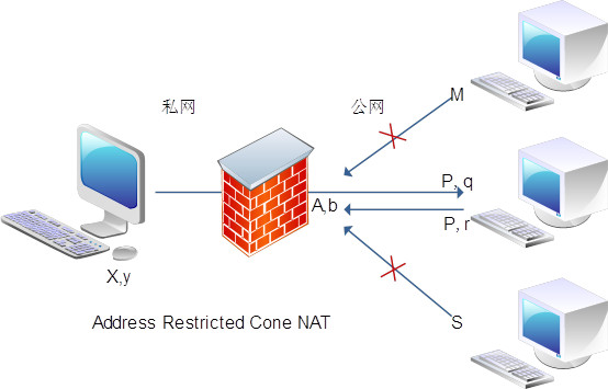
Restricted Cone NAT - 限锥 NAT:
同一个内网 Endpoint1 出站请求均被 NAT 映射成同一个外网 Endpoint2,但是只有 Endpoint1 曾经出站连接过的外部主机才能进行入站连接,只判断外网主机的 IP 地址。这意味着,NAT 设备只向内转发那些来自于当前已知的外部主机的数据包,从而保障了外部请求来源的安全性。
-
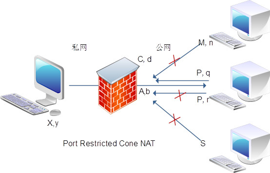
Port Restricted Cone NAT - 端口限锥 NAT:
与限锥 NAT 很相似,但是对端口作进一步限制。只有内网 Endpoint1 曾经出站连接过的外网主机 Endpoint3 (外网主机对应的 IP 和端口)。通过进一步约束 PORT,强化了对外部报文请求来源的限制,增强了安全性。
-
Symmetric NAT - 对称 NAT:
以上三种 Cone NAT,映射关系只和内网 Endpoint1 相关,只要 Endpoint1 不变,NAT 就都将其映射到同一个 Endpoint2。而对称 NAT 的映射关系不只与源 Endpoint1 相关,还与目的 Endpoint3 相关。也就是 Endpoint1 出站往目的 Endpoint3A,NAT 映射 Endpoint1 为 Endpoint2A;Endpoint1 发往目的 Endpoint3B 的请求,则被映射为 Endpoint2B。此外,只有经过内网主机出站连接的外网主机,才可以进行 UDP 入站连接。
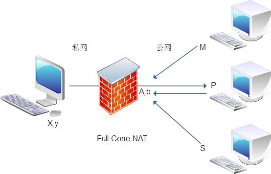
文档中使用 Cone 这个词来形容 NAT 的实现方式,可能是考虑“穿透”这个动作的形象,演示图中的外网主机到 NAT 的连线就是一个锥形。通常,确定 NAT 工作于什么方式非常重要,不同方式决定了如何实现 NAT 穿透。
以上是 RFC 3489 Classic STUN 文档描述,最新的 RFC 8489 已经不使用这样的分类描述,并且 STUN 这个词的语义也发生了变化 Simple 变 Session,STUN 从穿透解决方案变成 NAT 穿透解决方案中的工具,应该参考最新的 RFC 5128 P2P 协议文档。
从网络设备的实现上来看,NAT 映射可以按 Static、Dynamic 与 NAT、PAT 进行组合。静态方式由网络管理员配置指定映射关系,动态方式由设备临时指定映射关系。然后组合 IP 地址映射,或者端口映射,就有 4 种组合。
一般情况下,NAT 主要涉及修改出站数据包(outbound packet)的源 IP 地址的转换,将内部网络 IP 地址转换为外部网络的公共 IP 地址。或者修改入站数据包(inbound packet)的目标地址,将映射的公共 IP 地址修改为内网的 IP 地址。然而,有些情况需要对源地址和目标地址进行修改,这就需要 Twice NAT,相对于一般的 NAT 只修改单边的地址。
Twice NAT 的应用场景:
- 需要隐藏内网主机 IP 地址时,比如 VPN overlapping networks;
- 内部网络主机地址与外部网络上的主机地址重叠(overlapping),即不同网络中主机使用的 IP 地址相同;
- 多重地址转换:进行多次地址转换,将文经过多个转换节点,增加了网络的灵活性和扩展性。
- 跨网段通信:解决网段间的通信问题,使不同网段的主机能够互相访问。
下图演示了一次 DNS 请求过程中发生的 Twice NAT,原本 10.6.6.99 请求 DNS 服务器 8.8.8.8,但是经过 Twice NAT 映射后,数据包的源地址变为 NAT 设备的公网地址 32.8.2.55,目标地址变为另一台协同工作的 DNS 服务器 32.9.1.8:

内部网络主机地址与外部网络主机地址重叠的情况,NAT 会使用地址池中的临时地址替换 IP 包中的地址,解决内网地址与外网地址冲突问题。在数据包出站更换为临时地址,入站时再按映射关系修改回对应的真实地址。
Twice NAT is address translation where both source and destination IP addresses are modified due to addressing conflicts between two private realms. Two bi-directional NAT boxes connected together would essentially perform the same task, though a common address space that is not otherwise used by either private realm would be required.
Requirements for applications to work in the Twice NAT environment are the same as for Basic NAT. Addresses are mapped one to one.
参考 RFC 3235 NAT-Friendly Application Design Guidelines
RFC 5389 STUN 重新定义为 NAT 会话穿透工具,STUN - Session Traversal Utilities for NAT。STUN 本身不再是一种完整的 NAT 穿透解决方案,而是一种 NAT 穿透解决方案中的工具,也不再限定 UDP 是唯一支持的传输协议。因此将 RFC 3489 定义 STUN 称为经典 STUN(classic STUN)。
RFC 5128 P2P 协议文档更新了 NAT 的类型术语:
2. Terminology and Conventions Used ................................4
   2.1. Endpoint ...................................................5
   2.2. Endpoint Mapping ...........................................5
   2.3. Endpoint-Independent Mapping ...............................5
   2.4. Endpoint-Dependent Mapping .................................5
   2.5. Endpoint-Independent Filtering .............................6
   2.6. Endpoint-Dependent Filtering ...............................6
   2.7. P2P Application ............................................7
   2.8. NAT-Friendly P2P Application ...............................7
   2.9. Endpoint-Independent Mapping NAT (EIM-NAT) .................7
   2.10. Hairpinning ...............................................7
RFC 5128 P2P 协议文档 3. Techniques Used by P2P Applications to Traverse NATs 阐述了多种 NAT 穿透方法:
| Techniques Used to Traverse NATs | 说明 |
|---|---|
| Relaying | 服务器中继式穿透 |
| Connection Reversal | 逆向连接式穿透 |
| UDP Hole Punching | UDP 打洞穿透 |
| TCP Hole Punching | TCP 打洞穿透 |
| UDP Port Number Prediction | UDP 固定端口穿透 |
| TCP Port Number Prediction | TCP 固定端口穿透 |
UDP 打洞穿透是应用最广泛的一种,也是 NAT 设备提供支持最好的一种,它又细分三各情形:
- 通信双端由不同 NAT 隔离(Peers behind Different NATs)
- 通信双端在同一 NAT 之内(Peers behind the Same NAT)
- 通信双端由多层 NAT 隔离(Peers Separated by Multiple NATs)
服务器中继式穿透(Relaying)是可靠的穿透方式,但效率低下。需要一台拥有公网 IP 的服务器来执行中继服务。假设以下网络结构,服务器 S
                       Registry, Discovery
                       Combined with Relay
                             Server S
                        192.0.2.128:20001
                                 |
    +----------------------------+----------------------------+
    | ^ Registry/              ^   ^ Registry/              ^ |
    | | Relay-Req Session(A-S) |   | Relay-Req Session(B-S) | |
    | | 192.0.2.128:20001      |   |  192.0.2.128:20001     | |
    | | 192.0.2.1:62000        |   |  192.0.2.254:31000     | |
    |                                                         |
  +--------------+                                 +--------------+
  | 192.0.2.1    |                                 | 192.0.2.254  |
  |              |                                 |              |
  |    NAT A     |                                 |    NAT B     |
  +--------------+                                 +--------------+
    |                                                         |
    | ^ Registry/              ^   ^ Registry/              ^ |
    | | Relay-Req Session(A-S) |   | Relay-Req Session(B-S) | |
    | |  192.0.2.128:20001     |   |  192.0.2.128:20001     | |
    | |     10.0.0.1:1234      |   |     10.1.1.3:1234      | |
    |                                                         |
 Client A                                                 Client B
 10.0.0.1:1234                                        10.1.1.3:1234

     Figure 1: Use of a Relay Server to communicate with peers
逆向连接式穿透(Connection Reversal)应用在通信双端只有一端在 NAT 背后。假设以下网络结构,A 端主机要连接 B 端主机等同一般 C/S 构架的客户端连接。但是私网内的 B 端不能直接向 A 发起连接,因为它没有公网 IP 地址。这就需要一台拥有公网 IP 的约会服务器(Rendezvous Server)进行协调,NAT 背后的主机向它注册端点(endpoint),其它主机通过它发现 NAT 背后的主机。
注意“连接”一词,TCP 协议是基于连接的通信协议,一切来自还没有建立连接的主机的数据包都会被丢弃。但是,“连接”作为一个日常用语,它也可以表示发送数据包尝试建立连接的过程。
假设 A 端连接 S 服务器时,NAT 为 A 10.0.0.1:1234 分配了一个公网映射地址 192.0.2.1:62000,服务器通过建立的连接登记这个 A 端点的地址。B 就可以通过 S 向 A 中继一个链接请求,从而实现“逆向“地建立 A->B 之间的点对点链接。
如果 A 端没有建立与 S 的连接,没有执行 Registry Session(B-S) 这个过程,此时 B 端连接 192.0.2.1:62000 依然会失败,因为来自 B 的 TCP SYN 握手请求到达 NAT A 的时候会被拒绝,NAT A 还没有建立与私网主机的映射关系,只允许出站链接。
                      Registry and Discovery
                             Server S
                        192.0.2.128:20001
                                 |
    +----------------------------+----------------------------+
    | ^ Registry Session(A-S) ^     ^ Registry Session(B-S) ^ |
    | | 192.0.2.128:20001     |     |  192.0.2.128:20001    | |
    | | 192.0.2.1:62000       |     |  192.0.2.254:1234     | |
    |                                                         |
    | ^ P2P Session (A-B)     ^     |  P2P Session (B-A)    | |
    | | 192.0.2.254:1234      |     |  192.0.2.1:62000      | |
    | | 192.0.2.1:62000       |     v  192.0.2.254:1234     v |
    |                                                         |
  +--------------+                                            |
  | 192.0.2.1    |                                            |
  |              |                                            |
  |    NAT A     |                                            |
  +--------------+                                            |
    |                                                         |
    | ^ Registry Session(A-S) ^                               |
    | |  192.0.2.128:20001    |                               |
    | |     10.0.0.1:1234     |                               |
    |                                                         |
    | ^ P2P Session (A-B)     ^                               |
    | |  192.0.2.254:1234     |                               |
    | |     10.0.0.1:1234     |                               |
    |                                                         |
 Private Client A                                 Public Client B
 10.0.0.1:1234                                    192.0.2.254:1234

       Figure 2: Connection reversal using Rendezvous server
UPD 打洞穿透基于 Endpoint-Independent Mapping NAT (EIM-NAT) 设备。
有不少公开的 STUN 服务器,ping 测试通过,可以直接使用:
stun.l.google.com:19302
stun.stunprotocol.org
stun.minisipserver.com
stun.zoiper.com
stun.voipbuster.com
stun.sipgate.net
stun.schlund.de
stun.voipstunt.com
stun.1und1.de
stun.gmx.net
stun.callwithus.com
stun.internetcalls.com
stun.voip.aebc.com
stun.internetcalls.com
stun.callwithus.com
stun.gmx.net
stun.1und1.de
stun.voxgratia.org
https://www.fortinet.com/resources/cyberglossary/network-address-translation
Network address translation (NAT) is a technique commonly used by internet service providers (ISPs) and organizations to enable multiple devices to share a single public IP address. By using NAT, devices on a private network can communicate with devices on a public network without the need for each device to have its own unique IP address.
NAT was originally intended as a short-term solution to alleviate the shortage of available IPv4 addresses. By sharing a single IP address among multiple computers on a local network, NAT conserves the limited number of publicly routable IPv4 addresses. NAT also provides a layer of security for private networks because it hides devices' actual IP addresses behind a single public IP address.
One of the most common problems that can occur when setting up a home or office network is an Internet Protocol (IP) address conflict. [IP addresses] are assigned to each device on a network, and no two devices can have the same IP address. If two devices on the same network carry the same IP address, connection issues will arise.
There are a few ways you can avoid IP address conflicts. One is through network address translation (NAT).
NAT is typically implemented on a router, a device that connects two networks. When a device on the private network sends data to a device on the public network, the router intercepts the data and replaces the source IP address with its own public IP address. The router then sends the data to the destination device.
When the destination device sends data back to the router, the router intercepts this data and replaces the public IP address with the original source IP address. The router then sends the data to the original source device. This process is transparent to the devices on both networks.
To help you better visualize how NAT works, here are a few network address translation examples:
- A router connects a private network to the internet: The router, configured to use NAT, translates the private IP addresses of devices on the network into public IP addresses. This enables internal devices to communicate with devices on the internet, while remaining hidden from public view.
- An organization has multiple office locations and wants to connect them all using a private network: NAT can be used to translate the IP addresses of devices on each network so they can communicate with one another as if they were on the same network. This allows the company to keep its internal network private and secure, while allowing employees at different locations to communicate with each other.
Network address translation offers multiple significant benefits:
- IP address conservation: By enabling multiple devices to share a single IP address, NAT helps conserve IP address space. This is especially important for organizations that have been assigned a limited number of IP addresses by their ISP.
- Improved security: NAT can provide a measure of security by hiding the internal network from the outside world. This can be useful for preventing attacks that target specific IP addresses or for preventing devices on the internal network from being accessed directly from the internet. NAT can also help prevent devices on the internal network from accessing malicious or unwanted websites.
- Better speed: NAT can improve communication speed by reducing the number of packets that need to be routed through the network. This is because NAT eliminates the need for each device on the internal network to have its own unique IP address.
- Flexibility: NAT can also be used to provide flexibility in network design, which is particularly useful for organizations that want to change their network configuration without changing their IP addresses. Organizations may want to change their network configuration to improve security or performance or to add new devices to the network.
- **Multi-homing:**NAT can be used to allow devices on a private network to connect to multiple public networks, a network configuration practice called multi-homing. This can be valuable for organizations that want to connect to multiple ISPs or that want to provide [failover] in case one of the ISPs goes down. Multi-homing with NAT provides connection redundancy and increases uptime by allowing traffic to be routed through multiple ISPs.
- Cost savings: NAT reduces the number of IP addresses an organization needs, which can save them money on IP address licenses and other associated costs.
- Easier network administration: NAT makes it easier to manage a network by reducing the number of IP addresses that need to be assigned. This benefits organizations with a large fleet of devices and those that want to reduce the amount of time and effort required to manage their networks.
There are three network address translation types:
In static NAT, every internal IP address is mapped to a unique external IP address. This is one-to-one mapping. When outgoing traffic arrives at the router, the router replaces the destination IP address with the mapped global IP. When the return traffic comes back to the router, the router replaces the mapped global IP address with the source IP address.
Static NAT is mostly used in servers that need to be accessible from the internet, such as web servers and email servers.
In dynamic network address translation, internal IP addresses are mapped to a pool of external IP addresses. This is one-to-many mapping. When the outgoing traffic arrives at the router, the router replaces the destination IP address with a free global IP address from the pool. When the return traffic comes back to the router, the router replaces the mapped global IP address with the source IP address.
Dynamic NAT is mostly used in networks that need outbound internet connectivity.
PAT is a type of dynamic NAT that maps multiple internal IP addresses to a single external IP address via port numbers. This is many-to-one mapping. When a computer connects to the internet, the router assigns it a port number that it then appends to the computer's internal IP address, in turn giving the computer a unique IP address. When a second computer connects to the internet, it gets the same external IP address but a different port number.
PAT is mostly used in home networks.
One way that NAT can help improve network security is by hiding internal IP addresses from external users. This makes it more difficult for attackers to target specific devices on the network.
Another way that NAT can improve security is by providing a level of traffic filtering. By controlling which internal IP addresses are mapped to external IP addresses, NAT can be used to block certain types of traffic from reaching internal systems. For example, an organization can use NAT to block all inbound traffic from a specific IP address or range of IP addresses that are known to be associated with malicious activity.
NAT can also help improve [network security] by making it easier to track and manage network traffic. By mapping internal IP addresses to a single external IP address, NAT can simplify the process of tracking and logging network activity. This can be helpful for identifying suspicious or unusual activity on the network.
The [Fortinet Security Fabric] offers a unified, integrated approach to security to enable organizations to better protect their networks from a variety of threats. It includes several built-in features, such as:
- A NAT engine for hiding internal IP addresses and providing a level of traffic filtering
- A traffic monitoring system to track and log network activity
- An intrusion prevention system for detecting and blocking suspicious traffic
Fortinet also boosts network security through the [FortiGate Next-Generation Firewall] (NGFW), which provides complete visibility and threat protection across your organization.
Network address translation (NAT) is a technique commonly used by internet service providers (ISPs) and organizations to enable multiple devices to share a single public IP address. By using NAT, devices on a private network can communicate with devices on a public network without the need for each device to have its own unique IP address.
The three main NAT types are static NAT, dynamic NAT, and port address translation (PAT).
When a device on the private network sends data to a device on the public network, the router intercepts the data and replaces the source IP address with its own public IP address. The router then sends the data to the destination device. When the destination device responds by sending data back to the router, the router intercepts this data and replaces the public IP address with the original source IP address. The router then sends the data to the original source device. This allows devices on a local network to communicate with devices on a public network without revealing their true IP addresses.
There are several benefits of using NAT. These include improved security, increased privacy, and improved network performance. NAT can also help conserve IP addresses by allowing multiple devices to share a single public IP address.
https://computer.howstuffworks.com/nat.htm
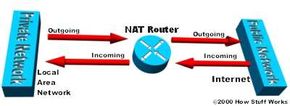
Network Address Translation helps improve security by reusing IP addresses. The NAT router translates traffic coming into and leaving the private network.
If you are reading this article, you are most likely connected to the Internet and viewing it at the HowStuffWorks Web site. There's a very good chance that you are using Network Address Translation (NAT) right now.
The Internet has grown larger than anyone ever imagined it could be. Although the exact size is unknown, the current estimate is that there are about 100 million hosts and more than 350 million users actively on the Internet. That is more than the entire population of the United States! In fact, the rate of growth has been such that the Internet is effectively doubling in size each year.
So what does the size of the Internet have to do with NAT? Everything! For a computer to communicate with other computers and [Web servers] on the Internet, it must have an IP address. An [IP address] (IP stands for Internet Protocol) is a unique 32-bit number that identifies the location of your computer on a network. Basically, it works like your street address -- as a way to find out exactly where you are and deliver information to you.
When IP addressing first came out, everyone thought that there were plenty of addresses to cover any need. Theoretically, you could have [4,294,967,296 unique addresses] (2^32). The actual number of available addresses is smaller (somewhere between 3.2 and 3.3 billion) because of the way that the addresses are separated into classes, and because some addresses are set aside for multicasting, testing or other special uses.
With the explosion of the Internet and the increase in [home networks] and business networks, the number of available IP addresses is simply not enough. The obvious solution is to redesign the address format to allow for more possible addresses. This is being developed (called IPv6), but will take several years to implement because it requires modification of the entire infrastructure of the Internet.
This is where NAT (RFC 1631) comes to the rescue. Network Address Translation allows a single device, such as a [router], to act as an agent between the Internet (or "public network") and a local (or "private") network. This means that only a single, unique IP address is required to represent an entire group of computers.
But the shortage of IP addresses is only one reason to use NAT. In this article, you will learn more about how NAT can benefit you. But first, let's take a closer look at NAT and exactly what it can do...
Contents
- What Does NAT Do?
- NAT Configuration
- Dynamic NAT and Overloading
- Stub Domains
- Security and Administration
- Multi-homing
NAT is like the receptionist in a large office. Let's say you have left instructions with the receptionist not to forward any calls to you unless you request it. Later on, you call a potential client and leave a message for that client to call you back. You tell the receptionist that you are expecting a call from this client and to put her through.
The client calls the main number to your office, which is the only number the client knows. When the client tells the receptionist that she is looking for you, the receptionist checks a lookup table that matches your name with your extension. The receptionist knows that you requested this call, and therefore forwards the caller to your extension.
Developed by Cisco, Network Address Translation is used by a device ([firewall], [router] or computer that sits between an internal network and the rest of the world. NAT has many forms and can work in several ways:

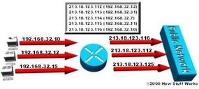
In static NAT, the computer with the IP address of 192.168.32.10 will always translate to 213.18.123.110.
- Static NAT - Mapping an unregistered IP address to a registered IP address on a one-to-one basis. Particularly useful when a device needs to be accessible from outside the network.
In dynamic NAT, the computer with the IP address 192.168.32.10 will translate to the first available address in the range from 213.18.123.100 to 213.18.123.150.
-
Dynamic NAT - Maps an unregistered IP address to a registered IP address from a group of registered IP addresses.
-
Overloading - A form of dynamic NAT that maps multiple unregistered IP addresses to a single registered IP address by using different ports. This is known also as PAT (Port Address Translation), single address NAT or port-level multiplexed NAT.
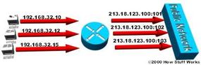
In overloading, each computer on the private network is translated to the same IP address (213.18.123.100), but with a different port number assignment.
- Overlapping - When the IP addresses used on your internal network are registered IP addresses in use on another network, the router must maintain a lookup table of these addresses so that it can intercept them and replace them with registered unique IP addresses. It is important to note that the NAT router must translate the "internal" addresses to registered unique addresses as well as translate the "external" registered addresses to addresses that are unique to the private network. This can be done either through static NAT or by using DNS and implementing dynamic NAT.
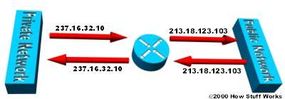
The internal IP range (237.16.32.xx) is also a registered range used by another network. Therefore, the router is translating the addresses to avoid a potential conflict with another network. It will also translate the registered global IP addresses back to the unregistered local IP addresses when information is sent to the internal network.
The internal network is usually a LAN (Local Area Network), commonly referred to as the stub domain. A stub domain is a LAN that uses IP addresses internally. Most of the network traffic in a stub domain is local, so it doesn't travel outside the internal network. A stub domain can include both registered and unregistered IP addresses. Of course, any computers that use unregistered IP addresses must use Network Address Translation to communicate with the rest of the world.
In the next section we'll look at the different ways NAT can be configured.
Thank You
Special thanks to Cisco for its support in creating this article.

IP addresses have different designations based on whether they are on the private network (stub domain) or on the public network (Internet), and whether the traffic is incoming or outgoing.
NAT can be configured in various ways. In the example below, the NAT router is configured to translate unregistered (inside, local) IP addresses, that reside on the private (inside) network, to registered IP addresses. This happens whenever a device on the inside with an unregistered address needs to communicate with the public (outside) network.
-
An ISP assigns a range of IP addresses to your company. The assigned block of addresses are registered, unique IP addresses and are called inside global addresses. Unregistered, private IP addresses are split into two groups. One is a small group (outside local addresses) that will be used by the NAT routers. The other, much larger group, known as inside local addresses, will be used on the stub domain. The outside local addresses are used to translate the unique IP addresses, known as outside global addresses, of devices on the public network.
-
Most computers on the stub domain communicate with each other using the inside local addresses.
-
Some computers on the stub domain communicate a lot outside the network. These computers have inside global addresses, which means that they do not require translation.
-
When a computer on the stub domain that has an inside local address wants to communicate outside the network, the packet goes to one of the NAT routers.
-
The NAT router checks the routing table to see if it has an entry for the destination address. If it does, the NAT router then translates the packet and creates an entry for it in the address translation table. If the destination address is not in the routing table, the packet is dropped.
-
Using an inside global address, the router sends the packet on to its destination.
-
A computer on the public network sends a packet to the private network. The source address on the packet is an outside global address. The destination address is an inside global address.
-
The NAT router looks at the address translation table and determines that the destination address is in there, mapped to a computer on the stub domain.
-
The NAT router translates the inside global address of the packet to the inside local address, and sends it to the destination computer.
NAT overloading utilizes a feature of the [TCP/IP protocol stack], multiplexing, that allows a computer to maintain several concurrent connections with a remote computer (or computers) using different [TCP or UDP] ports. An IP packet has a header that contains the following information:
- Source Address - The IP address of the originating computer, such as 201.3.83.132
- Source Port - The TCP or UDP port number assigned by the originating computer for this packet, such as Port 1080
- Destination Address - The IP address of the receiving computer, such as 145.51.18.223
- Destination Port - The TCP or UDP port number that the originating computer is asking the receiving computer to open, such as Port 3021
The addresses specify the two machines at each end, while the port numbers ensure that the connection between the two computers has a unique identifier. The combination of these four numbers defines a single TCP/IP connection. Each port number uses 16 bits, which means that there are a possible 65,536 (216) values. Realistically, since different manufacturers map the ports in slightly different ways, you can expect to have about 4,000 ports available.
Here's how dynamic NAT works:
- An internal network (stub domain) has been set up with IP addresses that were not specifically allocated to that company by IANA (Internet Assigned Numbers Authority), the global authority that hands out IP addresses. These addresses should be considered non-routable since they are not unique.
- The company sets up a NAT-enabled router. The router has a range of unique IP addresses given to the company by IANA.
- A computer on the stub domain attempts to connect to a computer outside the network, such as a Web server.
- The router receives the packet from the computer on the stub domain.
- The router saves the computer's non-routable IP address to an address translation table. The router replaces the sending computer's non-routable IP address with the first available IP address out of the range of unique IP addresses. The translation table now has a mapping of the computer's non-routable IP address matched with the one of the unique IP addresses.
- When a packet comes back from the destination computer, the router checks the destination address on the packet. It then looks in the address translation table to see which computer on the stub domain the packet belongs to. It changes the destination address to the one saved in the address translation table and sends it to that computer. If it doesn't find a match in the table, it drops the packet.
- The computer receives the packet from the router. The process repeats as long as the computer is communicating with the external system.
Here's how overloading works:
- An internal network (stub domain) has been set up with non-routable IP addresses that were not specifically allocated to that company by IANA.
- The company sets up a NAT-enabled router. The router has a unique IP address given to the company by IANA.
- A computer on the stub domain attempts to connect to a computer outside the network, such as a Web server.
- The router receives the packet from the computer on the stub domain.
- The router saves the computer's non-routable IP address and port number to an address translation table. The router replaces the sending computer's non-routable IP address with the router's IP address. The router replaces the sending computer's source port with the port number that matches where the router saved the sending computer's address information in the address translation table. The translation table now has a mapping of the computer's non-routable IP address and port number along with the router's IP address.
- When a packet comes back from the destination computer, the router checks the destination port on the packet. It then looks in the address translation table to see which computer on the stub domain the packet belongs to. It changes the destination address and destination port to the ones saved in the address translation table and sends it to that computer.
- The computer receives the packet from the router. The process repeats as long as the computer is communicating with the external system.
- Since the NAT router now has the computer's source address and source port saved to the address translation table, it will continue to use that same port number for the duration of the connection. A timer is reset each time the router accesses an entry in the table. If the entry is not accessed again before the timer expires, the entry is removed from the table.
In the next section we'll look at the organization of stub domains.
Look below to see how the computers on a stub domain might appear to external networks.
### Source Computer A
                             IP Address: 192.168.32.10
                          Computer Port: 400
                  NAT Router IP Address: 215.37.32.203
        NAT Router Assigned Port Number: 1


### Source Computer B
                             IP Address: 192.168.32.13
                          Computer Port: 50
                  NAT Router IP Address: 215.37.32.203
        NAT Router Assigned Port Number: 2


### Source Computer C
                             IP Address: 192.168.32.15
                          Computer Port: 3750
                  NAT Router IP Address: 215.37.32.203
        NAT Router Assigned Port Number: 3


### Source Computer D
                             IP Address: 192.168.32.18
                          Computer Port: 206
                  NAT Router IP Address: 215.37.32.203
        NAT Router Assigned Port Number: 4
As you can see, the NAT router stores the IP address and port number of each computer. It then replaces the IP address with its own registered IP address and the port number corresponding to the location, in the table, of the entry for that packet's source computer. So any external network sees the NAT router's IP address and the port number assigned by the router as the source-computer information on each packet.
You can still have some computers on the stub domain that use dedicated IP addresses. You can create an access list of IP addresses that tells the router which computers on the network require NAT. All other IP addresses will pass through untranslated.
The number of simultaneous translations that a router will support are determined mainly by the amount of DRAM (Dynamic Random Access Memory) it has. But since a typical entry in the address-translation table only takes about 160 bytes, a router with 4 MB of DRAM could theoretically process 26,214 simultaneous translations, which is more than enough for most applications.
IANA has set aside specific ranges of IP addresses for use as non-routable, internal network addresses. These addresses are considered unregistered (for more information check out RFC 1918: Address Allocation for Private Internets, which defines these address ranges). No company or agency can claim ownership of unregistered addresses or use them on public computers. Routers are designed to discard (instead of forward) unregistered addresses. What this means is that a packet from a computer with an unregistered address could reach a registered destination computer, but the reply would be discarded by the first router it came to.
There is a range for each of the three classes of IP addresses used for networking:
- Range 1: Class A - 10.0.0.0 through 10.255.255.255
- Range 2: Class B - 172.16.0.0 through 172.31.255.255
- Range 3: Class C - 192.168.0.0 through 192.168.255.255
Although each range is in a different class, your are not required to use any particular range for your internal network. It is a good practice, though, because it greatly diminishes the chance of an IP address conflict.

Static NAT (inbound mapping) allows a computer on the stub domain to maintain a specific address when communicating with devices outside the network.
Implementing dynamic NAT automatically creates a firewall between your internal network and outside networks, or between your internal network and the Internet. NAT only allows connections that originate inside the stub domain. Essentially, this means that a computer on an external network cannot connect to your computer unless your computer has initiated the contact. You can browse the Internet and connect to a site, and even download a file; but somebody else cannot latch onto your IP address and use it to connect to a port on your computer.
In specific circumstances, Static NAT, also called inbound mapping, allows external devices to initiate connections to computers on the stub domain. For instance, if you wish to go from an inside global address to a specific inside local address that is assigned to your Web server, Static NAT would enable the connection.
Some NAT routers provide for extensive filtering and traffic logging. Filtering allows your company to control what type of sites employees visit on the Web, preventing them from viewing questionable material. You can use traffic logging to create a log file of what sites are visited and generate various reports from it.
NAT is sometimes confused with proxy servers, but there are definite differences between them. NAT is transparent to the source and to destination computers. Neither one realizes that it is dealing with a third device. But a proxy server is not transparent. The source computer knows that it is making a request to the proxy server and must be configured to do so. The destination computer thinks that the proxy server IS the source computer, and deals with it directly. Also, proxy servers usually work at layer 4 (transport) of the OSI Reference Model or higher, while NAT is a layer 3 (network) protocol. Working at a higher layer makes proxy servers slower than NAT devices in most cases.
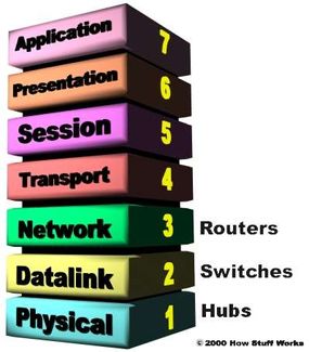
NAT operates at the Network layer (layer 3) of the OSI Reference Model -- this is the layer that routers work at.
A real benefit of NAT is apparent in network administration. For example, you can move your Web server or FTP server to another host computer without having to worry about broken links. Simply change the inbound mapping at the router to reflect the new host. You can also make changes to your internal network easily, because the only external IP address either belongs to the router or comes from a pool of global addresses.
NAT and DHCP (dynamic host configuration protocol ) are a natural fit. You can choose a range of unregistered IP addresses for your stub domain and have the DHCP server dole them out as necessary. It also makes it much easier to scale up your network as your needs grow. You don't have to request more IP addresses from IANA. Instead, you can just increase the range of available IP addresses configured in DHCP to immediately have room for additional computers on your network.
As businesses rely more and more on the Internet, having multiple points of connection to the Internet is fast becoming an integral part of their network strategy. Multiple connections, known as multi-homing, reduces the chance of a potentially catastrophic shutdown if one of the connections should fail.
In addition to maintaining a reliable connection, multi-homing allows a company to perform load-balancing by lowering the number of computers connecting to the Internet through any single connection. Distributing the load through multiple connections optimizes the performance and can significantly decrease wait times.
Multi-homed networks are often connected to several different ISPs (Internet Service Providers). Each ISP assigns an IP address (or range of IP addresses) to the company. Routers use BGP (Border Gateway Protocol), a part of the TCP/IP protocol suite, to route between networks using different protocols. In a multi-homed network, the router utilizes IBGP (Internal Border Gateway Protocol) on the stub domain side, and EBGP (External Border Gateway Protocol) to communicate with other routers.
Multi-homing really makes a difference if one of the connections to an ISP fails. As soon as the router assigned to connect to that ISP determines that the connection is down, it will reroute all data through one of the other routers.
NAT can be used to facilitate scalable routing for multi-homed, multi-provider connectivity. For more on multi-homing, see Cisco: Enabling Enterprise Multihoming.
For lots more information on NAT and related topics, check out the links on the next page.
A Network Address Translation or NAT is a mapping method of providing internet connection to local servers and hosts. In NAT, you take several local IPs and map them to one single global IP to transmit information across a routing device.
NAT only affects a little bit of your internet speed. It is barely noticeable if you’re using a reasonable router for translating your IPs.
With NAT enabled, it is easier to re-use your personal IP addresses with extra security. Moreover, NAT allows you to keep your external and internal IP addresses private and secure. You can also save the memory of your IP address by connecting several hosts via the internet using only a few external IPs.
NAT stands for Network Address Translation while PAT stands for Port Address Translation. As the names suggest, both NAT and PAT are used to translate private IPs into public IPs to save space and connect multiple devices. The difference is that PAT uses port numbers to map IP addresses whereas NAT doesn’t.
There are many forms of NAT. Static NAT maps an unregistered IP address to a registered IP address on a one-to-one basis; Dynamic NAT maps an unregistered IP address to a registered IP address from a group of registered IP addresses; Overloading maps multiple unregistered IP addresses to a single registered IP address by using different ports; Overlapping happens when a device on one network is assigned an IP address on the same subnet as another device on the internet or external network.
- How Web Servers Work
- How LAN Switches Work
- How Routers Work
- How Ethernet Works
- How Home Networking Works
- How OSI Works
- Network Address Translation FAQ
- Netsizer: Realtime Internet Growth
- Cisco: Network Address Translation
- NAT Technical Discussion
- Cisco: Configuring IP Addressing
- Cisco: NAT Overlapping
- Cisco: NAT Order of Operation
- IP Journal: The Trouble With NAT
- Cisco: Enabling Enterprise Multihoming
- RFC 1631: The IP Network Address Translator (NAT)
- RFC 1918: Address Allocation for Private Internets
Cite This!
Please copy/paste the following text to properly cite this HowStuffWorks.com article:
Copy
Jeff Tyson "How Network Address Translation Works" 2 February 2001.
HowStuffWorks.com. https://computer.howstuffworks.com/nat.htm 18 March 2024
- https://tailscale.com/blog/how-nat-traversal-works
- NAT 穿透是如何工作的:技术原理及企业级实践 https://zhuanlan.zhihu.com/p/450235047
August 21 2020 David Anderson
Contents
- Figuring out firewalls
- The nature of NATs
- NAT notes for nerds
- Integrating it all with ICE
- Concluding our connectivity chat
We covered a lot of ground in our post about How Tailscale Works. However, we glossed over how we can get through NATs (Network Address Translators) and connect your devices directly to each other, no matter what’s standing between them. Let’s talk about that now!
Let’s start with a simple problem: establishing a peer-to-peer connection between two machines. In Tailscale’s case, we want to set up a WireGuard® tunnel, but that doesn’t really matter. The techniques we use are widely applicable and the work of many people over decades. For example, WebRTC uses this bag of tricks to send peer-to-peer audio, video and data between web browsers. VoIP phones and some video games use similar techniques, though not always successfully.
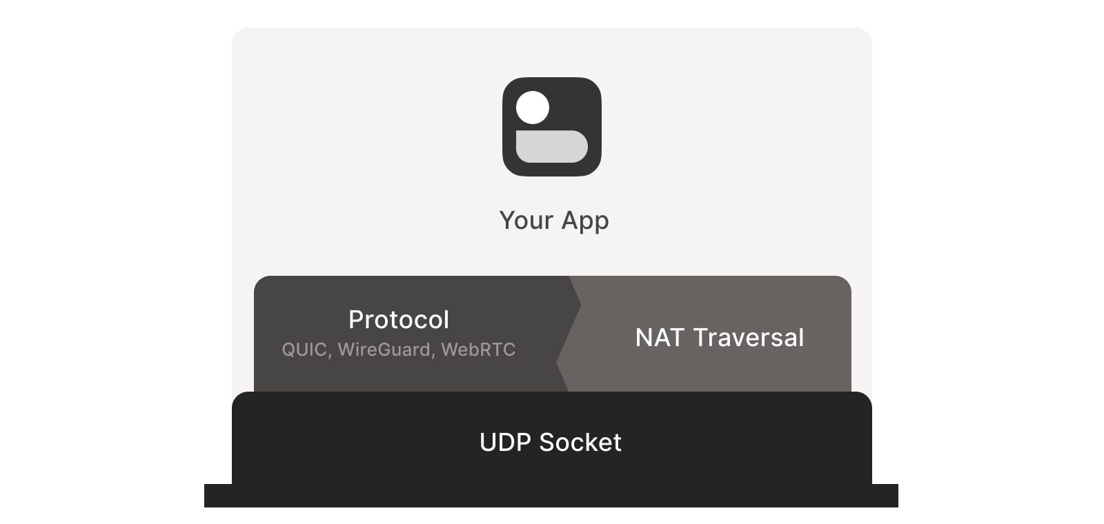
We’ll be discussing these techniques generically, using Tailscale and others for examples where appropriate. Let’s say you’re making your own protocol and that you want NAT traversal. You need two things.
First, the protocol should be based on UDP. You can do NAT traversal with TCP, but it adds another layer of complexity to an already quite complex problem, and may even require kernel customizations depending on how deep you want to go. We’re going to focus on UDP for the rest of this article.
If you’re reaching for TCP because you want a stream-oriented connection when the NAT traversal is done, consider using QUIC instead. It builds on top of UDP, so we can focus on UDP for NAT traversal and still have a nice stream protocol at the end.
Second, you need direct control over the network socket that’s sending and receiving network packets. As a rule, you can’t take an existing network library and make it traverse NATs, because you have to send and receive extra packets that aren’t part of the “main” protocol you’re trying to speak. Some protocols tightly integrate the NAT traversal with the rest (e.g. WebRTC). But if you’re building your own, it’s helpful to think of NAT traversal as a separate entity that shares a socket with your main protocol. Both run in parallel, one enabling the other.
Direct socket access may be tough depending on your situation. One workaround is to run a local proxy. Your protocol speaks to this proxy, and the proxy does both NAT traversal and relaying of your packets to the peer. This layer of indirection lets you benefit from NAT traversal without altering your original program.
With prerequisites out of the way, let’s go through NAT traversal from first principles. Our goal is to get UDP packets flowing bidirectionally between two devices, so that our other protocol (WireGuard, QUIC, WebRTC, …) can do something cool. There are two obstacles to having this Just Work: stateful firewalls and NAT devices.
Stateful firewalls are the simpler of our two problems. In fact, most NAT devices include a stateful firewall, so we need to solve this subset before we can tackle NATs.
There are many incarnations to consider. Some you might recognize are the Windows Defender firewall, Ubuntu’s ufw (using iptables/nftables), BSD’s pf (also used by macOS) and AWS’s Security Groups. They’re all very configurable, but the most common configuration allows all “outbound” connections and blocks all “inbound” connections. There might be a few handpicked exceptions, such as allowing inbound SSH.
But connections and “direction” are a figment of the protocol designer’s imagination. On the wire, every connection ends up being bidirectional; it’s all individual packets flying back and forth. How does the firewall know what’s inbound and what’s outbound?
That’s where the stateful part comes in. Stateful firewalls remember what packets they’ve seen in the past and can use that knowledge when deciding what to do with new packets that show up.
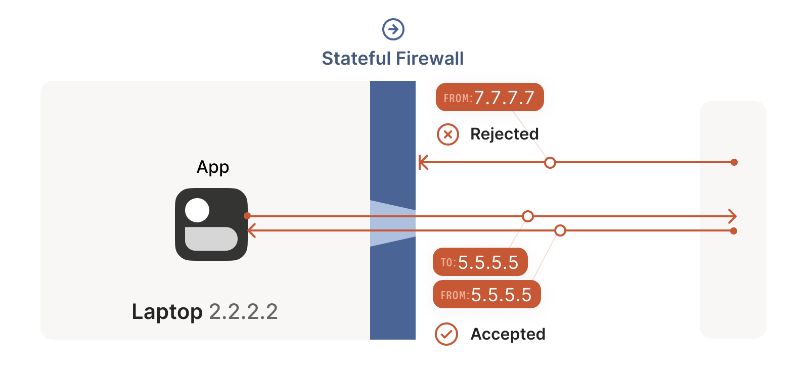
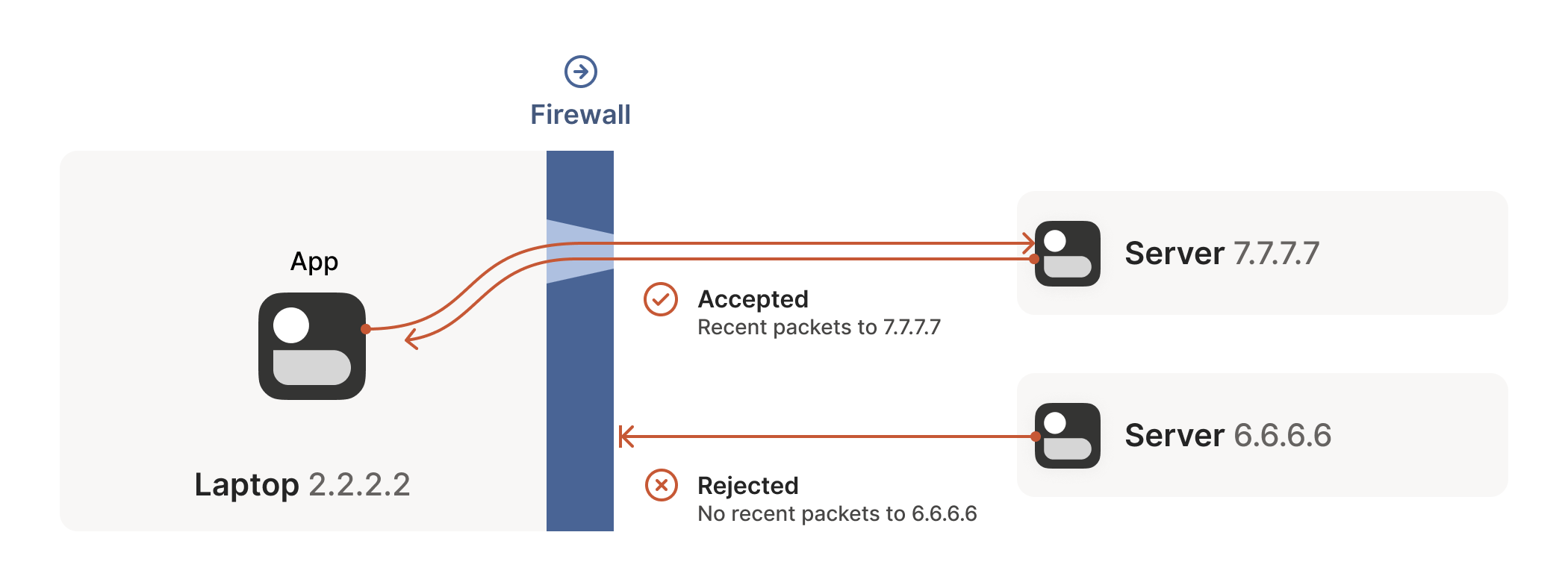
For UDP, the rule is very simple: the firewall allows an inbound UDP packet if it previously saw a matching outbound packet. For example, if our laptop firewall sees a UDP packet leaving the laptop from 2.2.2.2:1234 to 7.7.7.7:5678, it’ll make a note that incoming packets from 7.7.7.7:5678 to 2.2.2.2:1234 are also fine. The trusted side of the world clearly intended to communicate with 7.7.7.7:5678, so we should let them talk back.
(As an aside, some very relaxed firewalls might allow traffic from anywhere back to 2.2.2.2:1234 once 2.2.2.2:1234 has communicated with anyone. Such firewalls make our traversal job easier, but are increasingly rare.)
This rule for UDP traffic is only a minor problem for us, as long as all the firewalls on the path are “facing” the same way. That’s usually the case when you’re communicating with a server on the internet. Our only constraint is that the machine that’s behind the firewall must be the one initiating all connections. Nothing can talk to it, unless it talks first.
This is fine, but not very interesting: we’ve reinvented client/server communication, where the server makes itself easily reachable to clients. In the VPN world, this leads to a hub-and-spoke topology: the hub has no firewalls blocking access to it and the firewalled spokes connect to the hub.
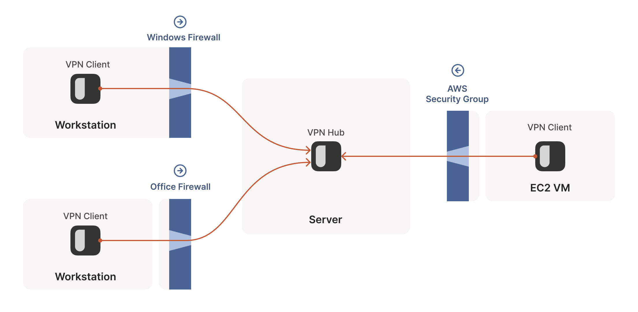
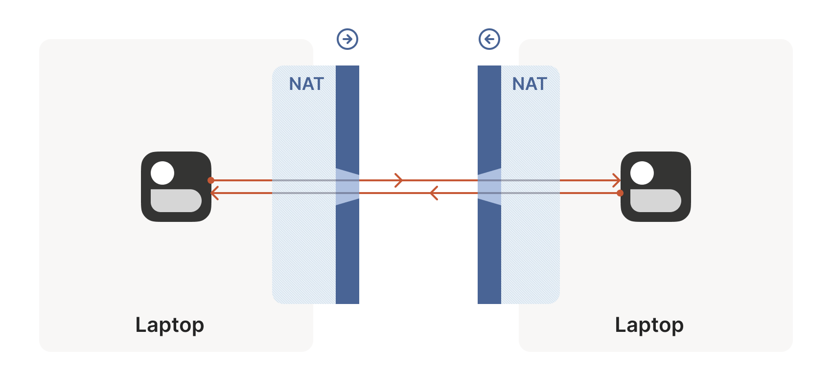
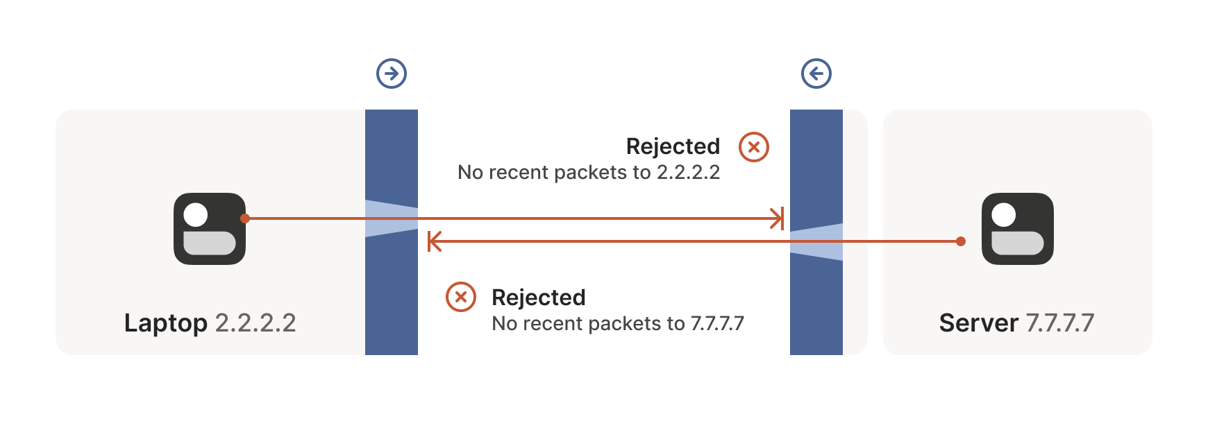
The problems start when two of our “clients” want to talk directly. Now the firewalls are facing each other. According to the rule we established above, this means both sides must go first, but also that neither can go first, because the other side has to go first!
How do we get around this? One way would be to require users to reconfigure one or both of the firewalls to “open a port” and allow the other machine’s traffic. This is not very user friendly. It also doesn’t scale to mesh networks like Tailscale, in which we expect the peers to be moving around the internet with some regularity. And, of course, in many cases you don’t have control over the firewalls: you can’t reconfigure the router in your favorite coffee shop, or at the airport. (At least, hopefully not!)
We need another option. One that doesn’t involve reconfiguring firewalls.
The trick is to carefully read the rule we established for our stateful firewalls. For UDP, the rule is: packets must flow out before packets can flow back in.
However, nothing says the packets must be related to each other beyond the IPs and ports lining up correctly. As long as some packet flowed outwards with the right source and destination, any packet that looks like a response will be allowed back in, even if the other side never received your packet!
So, to traverse these multiple stateful firewalls, we need to share some information to get underway: the peers have to know in advance the ip:port their counterpart is using. One approach is to statically configure each peer by hand, but this approach doesn’t scale very far. To move beyond that, we built a coordination server to keep the ip:port information synchronized in a flexible, secure manner.
Then, the peers start sending UDP packets to each other. They must expect some of these packets to get lost, so they can’t carry any precious information unless you’re prepared to retransmit them. This is generally true of UDP, but especially true here. We’re going to lose some packets in this process.
Our laptop and workstation are now listening on fixed ports, so that they both know exactly what ip:port to talk to. Let’s take a look at what happens.
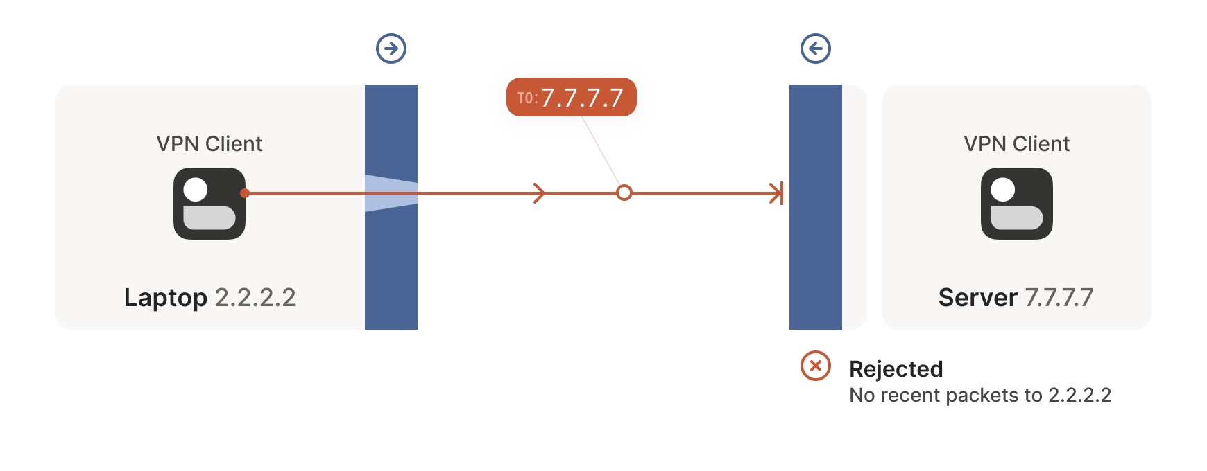
The laptop’s first packet, from 2.2.2.2:1234 to 7.7.7.7:5678, goes through the Windows Defender firewall and out to the internet. The corporate firewall on the other end blocks the packet, since it has no record of 7.7.7.7:5678 ever talking to 2.2.2.2:1234. However, Windows Defender now remembers that it should expect and allow responses from 7.7.7.7:5678 to 2.2.2.2:1234.
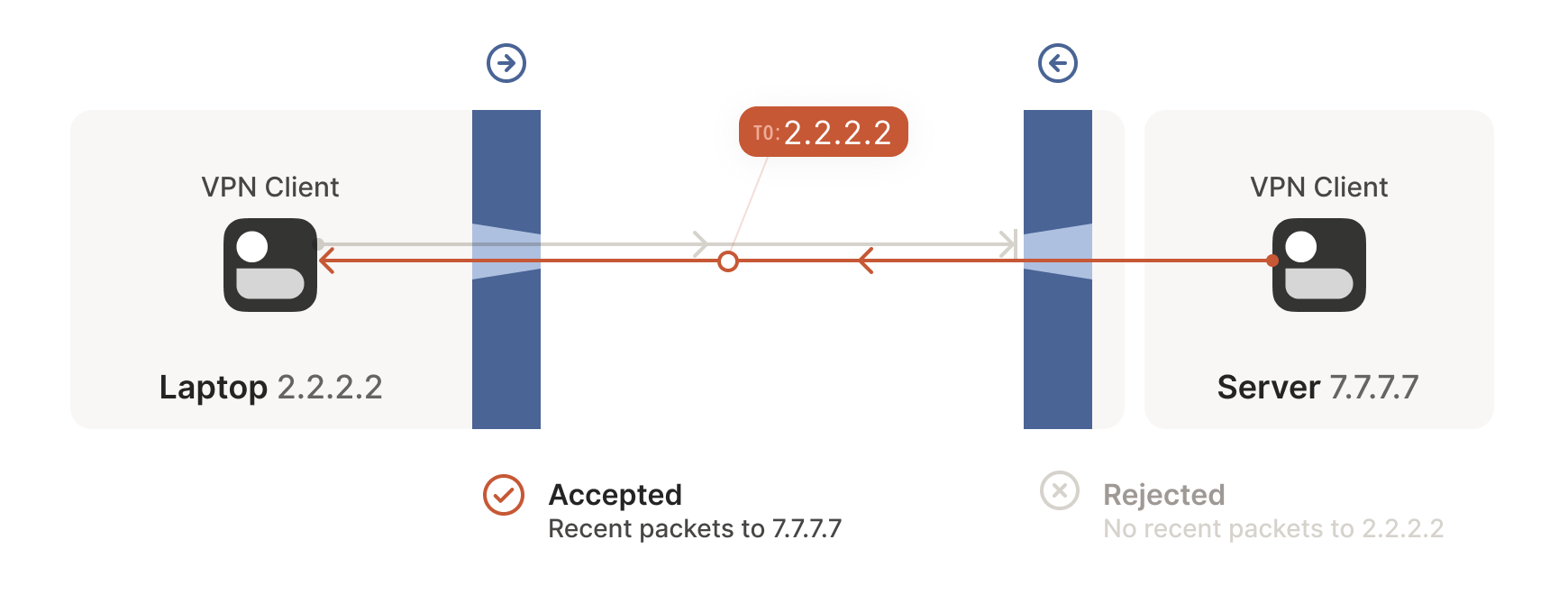
Next, the workstation’s first packet from 7.7.7.7:5678 to 2.2.2.2:1234 goes through the corporate firewall and across the internet. When it arrives at the laptop, Windows Defender thinks “ah, a response to that outbound request I saw”, and lets the packet through! Additionally, the corporate firewall now remembers that it should expect responses from 2.2.2.2:1234 to 7.7.7.7:5678, and that those packets are also okay.
Encouraged by the receipt of a packet from the workstation, the laptop sends another packet back. It goes through the Windows Defender firewall, through the corporate firewall (because it’s a “response” to a previously sent packet), and arrives at the workstation.
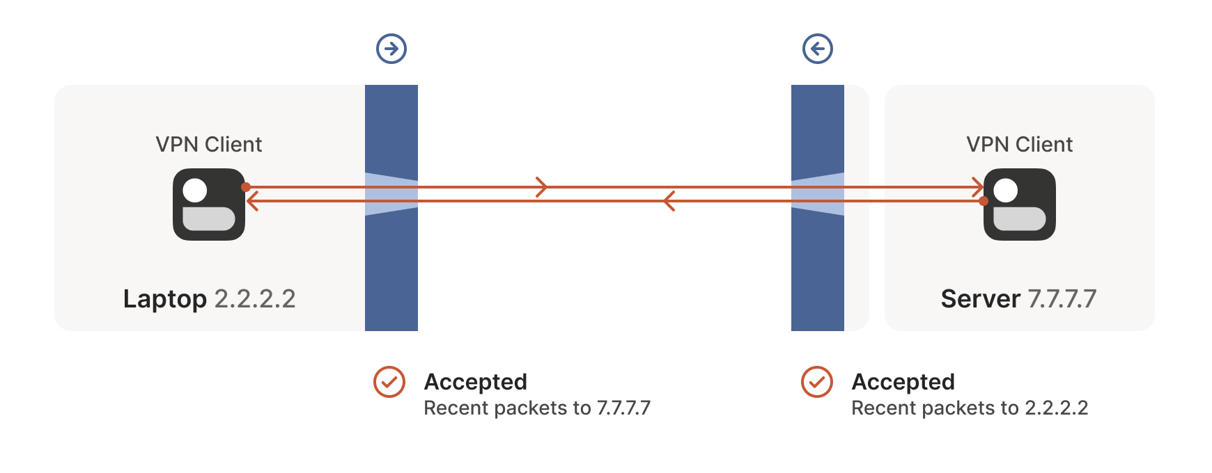
Success! We’ve established two-way communication through a pair of firewalls that, at first glance, would have prevented it.
It’s not always so easy. We’re relying on some indirect influence over third-party systems, which requires careful handling. What do we need to keep in mind when managing firewall-traversing connections?
Both endpoints must attempt communication at roughly the same time, so that all the intermediate firewalls open up while both peers are still around. One approach is to have the peers retry continuously, but this is wasteful. Wouldn’t it be better if both peers knew to start establishing a connection at the same time?
This may sound a little recursive: to communicate, first you need to be able to communicate. However, this preexisting “side channel” doesn’t need to be very fancy: it can have a few seconds of latency, and only needs to deliver a few thousand bytes in total, so a tiny VM can easily be a matchmaker for thousands of machines.
In the distant past, I used XMPP chat messages as the side channel, with great results. As another example, WebRTC requires you to come up with your own “signalling channel” (a name that reveals WebRTC’s IP telephony ancestry), and plug it into the WebRTC APIs. In Tailscale, our coordination server and fleet of DERP (Detour Encrypted Routing Protocol) servers act as our side channel.
Stateful firewalls have limited memory, meaning that we need periodic communication to keep connections alive. If no packets are seen for a while (a common value for UDP is 30 seconds), the firewall forgets about the session, and we have to start over. To avoid this, we use a timer and must either send packets regularly to reset the timers, or have some out-of-band way of restarting the connection on demand.
On the plus side, one thing we don’t need to worry about is exactly how many firewalls exist between our two peers. As long as they are stateful and allow outbound connections, the simultaneous transmission technique will get through any number of layers. That’s really nice, because it means we get to implement the logic once, and it’ll work everywhere.
…Right?
Well, not quite. For this to work, our peers need to know in advance what ip:port to use for their counterparts. This is where NATs come into play, and ruin our fun.
We can think of NAT (Network Address Translator) devices as stateful firewalls with one more really annoying feature: in addition to all the stateful firewalling stuff, they also alter packets as they go through.
A NAT device is anything that does any kind of Network Address Translation, i.e. altering the source or destination IP address or port. However, when talking about connectivity problems and NAT traversal, all the problems come from Source NAT, or SNAT for short. As you might expect, there is also DNAT (Destination NAT), and it’s very useful but not relevant to NAT traversal.
The most common use of SNAT is to connect many devices to the internet, using fewer IP addresses than the number of devices. In the case of consumer-grade routers, we map all devices onto a single public-facing IP address. This is desirable because it turns out that there are way more devices in the world that want internet access, than IP addresses to give them (at least in IPv4 — we’ll come to IPv6 in a little bit). NATs let us have many devices sharing a single IP address, so despite the global shortage of IPv4 addresses, we can scale the internet further with the addresses at hand.
Let’s look at what happens when your laptop is connected to your home Wi-Fi and talks to a server on the internet.
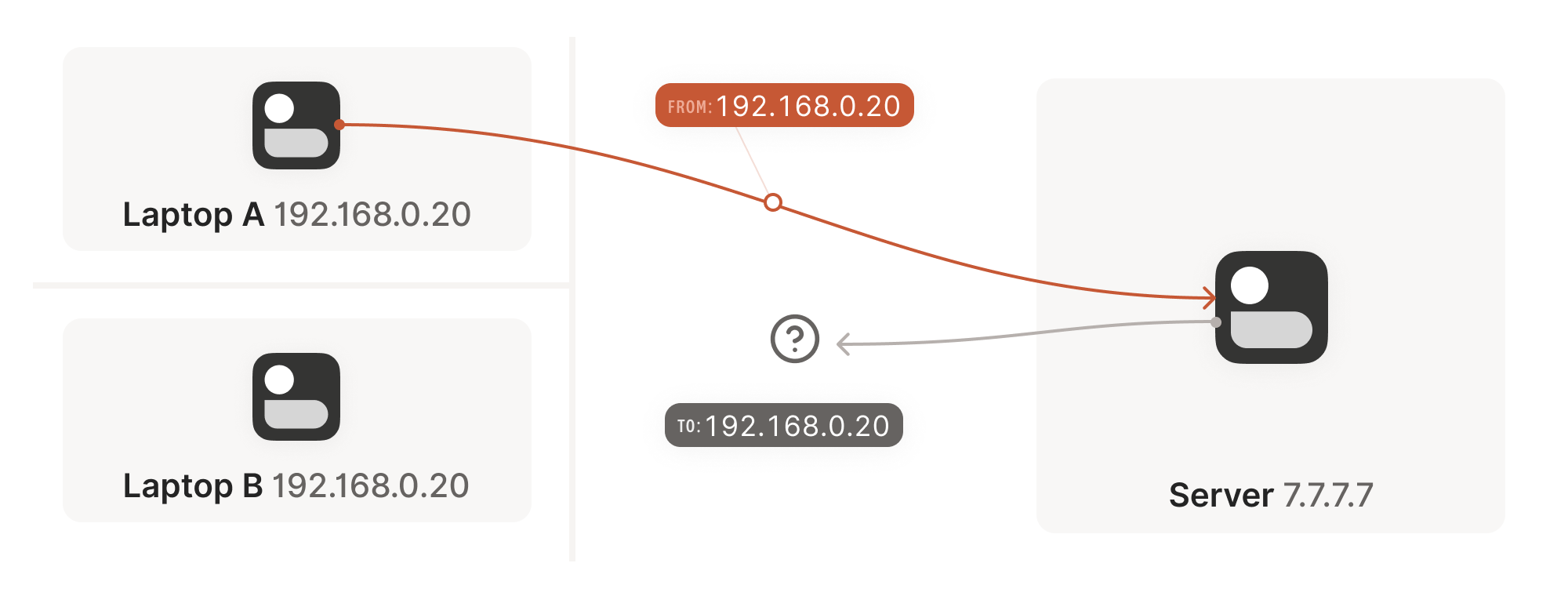
Your laptop sends UDP packets from 192.168.0.20:1234 to 7.7.7.7:5678. This is exactly the same as if the laptop had a public IP. But that won’t work on the internet: 192.168.0.20 is a private IP address, which appears on many different peoples’ private networks. The internet won’t know how to get responses back to us.
Enter the home router. The laptop’s packets flow through the home router on their way to the internet, and the router sees that this is a new session that it’s never seen before.
It knows that 192.168.0.20 won’t fly on the internet, but it can work around that: it picks some unused UDP port on its own public IP address — we’ll use 2.2.2.2:4242 — and creates a NAT mapping that establishes an equivalence: 192.168.0.20:1234 on the LAN side is the same as 2.2.2.2:4242 on the internet side.
From now on, whenever it sees packets that match that mapping, it will rewrite the IPs and ports in the packet appropriately.
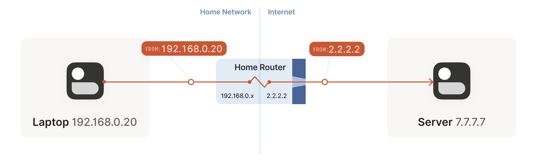
Resuming our packet’s journey: the home router applies the NAT mapping it just created, and sends the packet onwards to the internet. Only now, the packet is from 2.2.2.2:4242, not 192.168.0.20:1234. It goes on to the server, which is none the wiser. It’s communicating with 2.2.2.2:4242, like in our previous examples sans NAT.
Responses from the server flow back the other way as you’d expect, with the home router rewriting 2.2.2.2:4242 back to 192.168.0.20:1234. The laptop is also none the wiser, from its perspective the internet magically figured out what to do with its private IP address.
Our example here was with a home router, but the same principle applies on corporate networks. The usual difference there is that the NAT layer consists of multiple machines (for high availability or capacity reasons), and they can have more than one public IP address, so that they have more public ip:port combinations to choose from and can sustain more active clients at once.
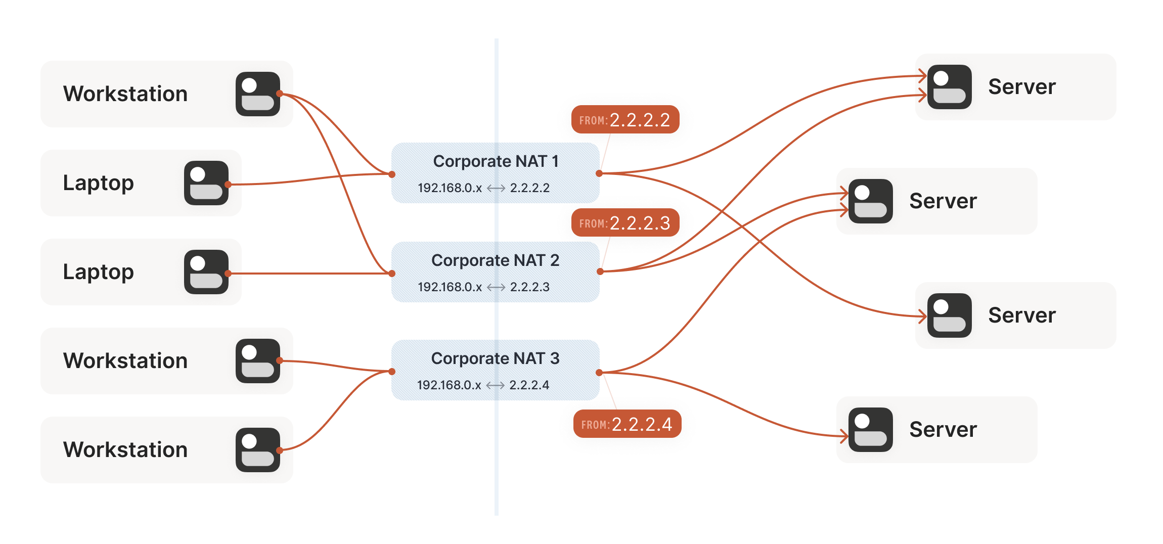
Multiple NATs on a single layer allow for higher availability or capacity, but function the same as a single NAT.
We now have a problem that looks like our earlier scenario with the stateful firewalls, but with NAT devices:
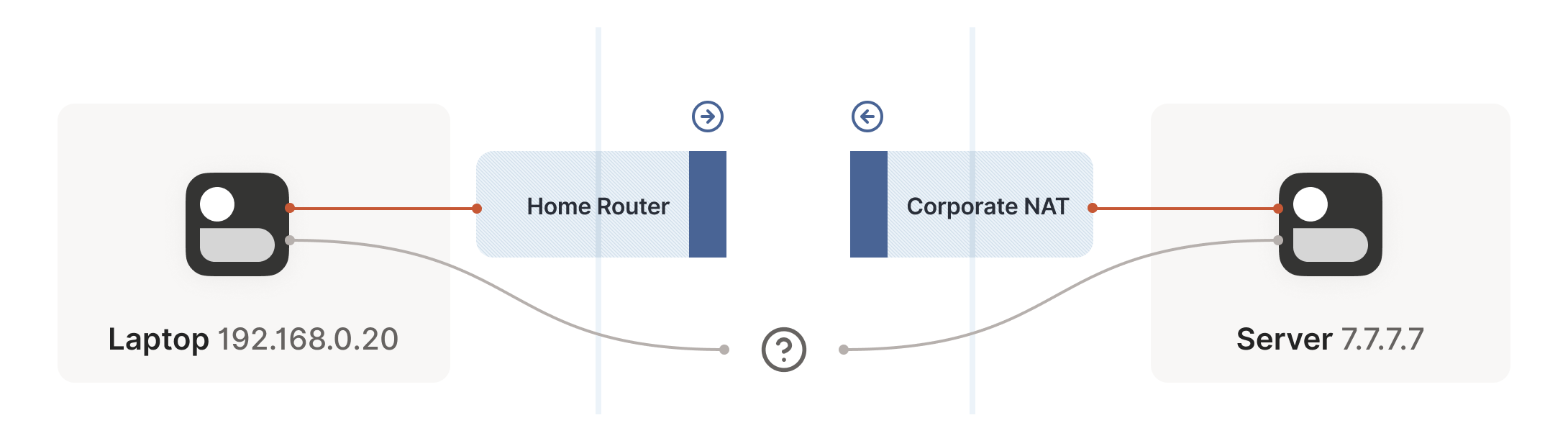
Our problem is that our two peers don’t know what the ip:port of their peer is. Worse, strictly speaking there is no ip:port until the other peer sends packets, since NAT mappings only get created when outbound traffic towards the internet requires it. We’re back to our stateful firewall problem, only worse: both sides have to speak first, but neither side knows to whom to speak, and can’t know until the other side speaks first.
How do we break the deadlock? That’s where STUN comes in. STUN is both a set of studies of the detailed behavior of NAT devices, and a protocol that aids in NAT traversal. The main thing we care about for now is the network protocol.
STUN relies on a simple observation: when you talk to a server on the internet from a NATed client, the server sees the public ip:port that your NAT device created for you, not your LAN ip:port. So, the server can tell you what ip:port it saw. That way, you know what traffic from your LAN ip:port looks like on the internet, you can tell your peers about that mapping, and now they know where to send packets! We’re back to our “simple” case of firewall traversal.
That’s fundamentally all that the STUN protocol is: your machine sends a “what’s my endpoint from your point of view?” request to a STUN server, and the server replies with “here’s the ip:port that I saw your UDP packet coming from.”
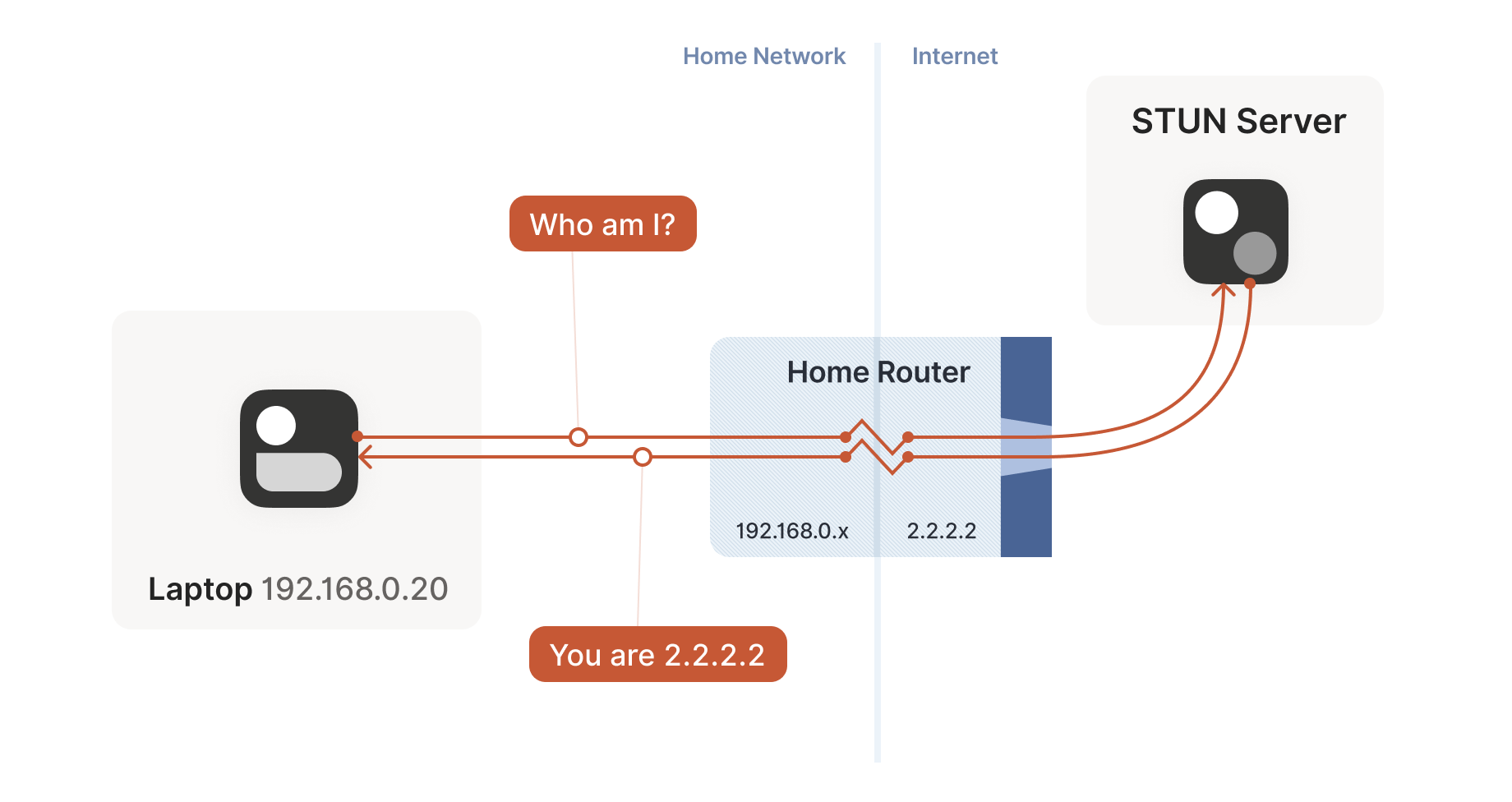
(The STUN protocol has a bunch more stuff in it — there’s a way of obfuscating the ip:port in the response to stop really broken NATs from mangling the packet’s payload, and a whole authentication mechanism that only really gets used by TURN and ICE, sibling protocols to STUN that we’ll talk about in a bit. We can ignore all of that stuff for address discovery.)
Incidentally, this is why we said in the introduction that, if you want to implement this yourself, the NAT traversal logic and your main protocol have to share a network socket. Each socket gets a different mapping on the NAT device, so in order to discover your public ip:port, you have to send and receive STUN packets from the socket that you intend to use for communication, otherwise you’ll get a useless answer.
Given STUN as a tool, it seems like we’re close to done. Each machine can do STUN to discover the public-facing ip:port for its local socket, tell its peers what that is, everyone does the firewall traversal stuff, and we’re all set… Right?
Well, it’s a mixed bag. This’ll work in some cases, but not others. Generally speaking, this’ll work with most home routers, and will fail with some corporate NAT gateways. The probability of failure increases the more the NAT device’s brochure mentions that it’s a security device. (NATs do not enhance security in any meaningful way, but that’s a rant for another time.)
The problem is an assumption we made earlier: when the STUN server told us that we’re 2.2.2.2:4242 from its perspective, we assumed that meant that we’re 2.2.2.2:4242 from the entire internet’s perspective, and that therefore anyone can reach us by talking to 2.2.2.2:4242.
As it turns out, that’s not always true. Some NAT devices behave exactly in line with our assumptions. Their stateful firewall component still wants to see packets flowing in the right order, but we can reliably figure out the correct ip:port to give to our peer and do our simultaneous transmission trick to get through. Those NATs are great, and our combination of STUN and the simultaneous packet sending will work fine with those.
(in theory, there are also NAT devices that are super relaxed, and don’t ship with stateful firewall stuff at all. In those, you don’t even need simultaneous transmission, the STUN request gives you an internet ip:port that anyone can connect to with no further ceremony. If such devices do still exist, they’re increasingly rare.)
Other NAT devices are more difficult, and create a completely different NAT mapping for every different destination that you talk to. On such a device, if we use the same socket to send to 5.5.5.5:1234 and 7.7.7.7:2345, we’ll end up with two different ports on 2.2.2.2, one for each destination. If you use the wrong port to talk back, you don’t get through.
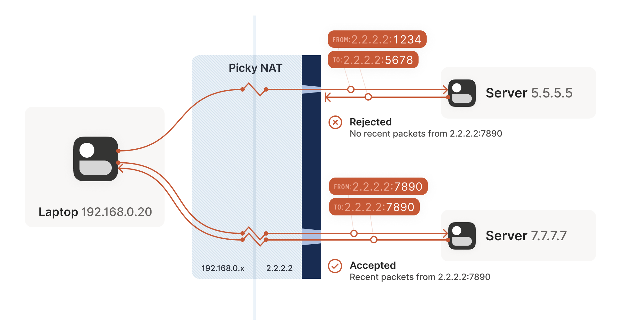
Now that we’ve discovered that not all NAT devices behave in the same way, we should talk terminology. If you’ve done anything related to NAT traversal before, you might have heard of “Full Cone”, “Restricted Cone”, “Port-Restricted Cone” and “Symmetric” NATs. These are terms that come from early research into NAT traversal.
That terminology is honestly quite confusing. I always look up what a Restricted Cone NAT is supposed to be. Empirically, I’m not alone in this, because most of the internet calls “easy” NATs Full Cone, when these days they’re much more likely to be Port-Restricted Cone.
More recent research and RFCs have come up with a much better taxonomy. First of all, they recognize that there are many more varying dimensions of behavior than the single “cone” dimension of earlier research, so focusing on the cone-ness of your NAT isn’t necessarily helpful. Second, they came up with words that more plainly convey what the NAT is doing.
The “easy” and “hard” NATs above differ in a single dimension: whether or not their NAT mappings depend on what the destination is. RFC 4787 calls the easy variant “Endpoint-Independent Mapping” (EIM for short), and the hard variant “Endpoint-Dependent Mapping” (EDM for short). There’s a subcategory of EDM that specifies whether the mapping varies only on the destination IP, or on both the destination IP and port. For NAT traversal, the distinction doesn’t matter. Both kinds of EDM NATs are equally bad news for us.
In the grand tradition of naming things being hard, endpoint-independent NATs still depend on an endpoint: each source ip:port gets a different mapping, because otherwise your packets would get mixed up with someone else’s packets, and that would be chaos. Strictly speaking, we should say “Destination Endpoint Independent Mapping” (DEIM?), but that’s a mouthful, and since “Source Endpoint Independent Mapping” would be another way to say “broken”, we don’t specify. Endpoint always means “Destination Endpoint.”
You might be wondering how 2 kinds of endpoint dependence maps into 4 kinds of cone-ness. The answer is that cone-ness encompasses two orthogonal dimensions of NAT behavior. One is NAT mapping behavior, which we looked at above, and the other is stateful firewall behavior. Like NAT mapping behavior, the firewalls can be Endpoint-Independent or a couple of variants of Endpoint-Dependent. If you throw all of these into a matrix, you can reconstruct the cone-ness of a NAT from its more fundamental properties:
=========================   =========================   =========================
                            Endpoint-Independent        Endpoint-Dependent
                            NAT mapping                 NAT mapping (all types)
=========================   =========================   =========================
Endpoint-Independent        Full Cone NAT               N/A*
firewall
=========================   =========================   =========================
Endpoint-Dependent          Restricted Cone NAT         N/A*
firewall (dest. IP only)
=========================   =========================   =========================
Endpoint-Dependent          Port-Restricted Cone NAT    Symmetric NAT
firewall (dest. IP+port)
=========================   =========================   =========================

* can theoretically exist, but don't show up in the wild
Once broken down like this, we can see that cone-ness isn’t terribly useful to us. The major distinction we care about is Symmetric versus anything else — in other words, we care about whether a NAT device is EIM or EDM.
While it’s neat to know exactly how your firewall behaves, we don’t care from the point of view of writing NAT traversal code. Our simultaneous transmission trick will get through all three variants of firewalls. In the wild we’re overwhelmingly dealing only with IP-and-port endpoint-dependent firewalls. So, for practical code, we can simplify the table down to:
=================   =========================   ===========================
                    Endpoint-Independent        Endpoint-Dependent
                    NAT mapping                 NAT mapping (dest. IP only)
=================   =========================   ===========================
Firewall is yes     Easy NAT                    Hard NAT
=================   =========================   ===========================
If you’d like to read more about the newer taxonomies of NATs, you can get the full details in RFCs 4787 (NAT Behavioral Requirements for UDP), 5382 (for TCP) and 5508 (for ICMP). And if you’re implementing a NAT device, these RFCs are also your guide to what behaviors you should implement, to make them well-behaved devices that play well with others and don’t generate complaints about Halo multiplayer not working.
Back to our NAT traversal. We were doing well with STUN and firewall traversal, but these hard NATs are a big problem. It only takes one of them in the whole path to break our current traversal plans.
But wait, this post is titled “how NAT traversal works”, not “how NAT traversal doesn’t work.” So presumably, I have a trick up my sleeve to get out of this, right?
This is a good time to have the awkward part of our chat: what happens when we empty our entire bag of tricks, and we still can’t get through? A lot of NAT traversal code out there gives up and declares connectivity impossible. That’s obviously not acceptable for us; Tailscale is nothing without the connectivity.
We could use a relay that both sides can talk to unimpeded, and have it shuffle packets back and forth. But wait, isn’t that terrible?
Sort of. It’s certainly not as good as a direct connection, but if the relay is “near enough” to the network path your direct connection would have taken, and has enough bandwidth, the impact on your connection quality isn’t huge. There will be a bit more latency, maybe less bandwidth. That’s still much better than no connection at all, which is where we were heading.
And keep in mind that we only resort to this in cases where direct connections fail. We can still establish direct connections through a lot of different networks. Having relays to handle the long tail isn’t that bad.
Additionally, some networks can break our connectivity much more directly than by having a difficult NAT. For example, we’ve observed that the UC Berkeley guest Wi-Fi blocks all outbound UDP except for DNS traffic. No amount of clever NAT tricks is going to get around the firewall eating your packets. So, we need some kind of reliable fallback no matter what.
You could implement relays in a variety of ways. The classic way is a protocol called TURN (Traversal Using Relays around NAT). We’ll skip the protocol details, but the idea is that you authenticate yourself to a TURN server on the internet, and it tells you “okay, I’ve allocated ip:port, and will relay packets for you.” You tell your peer the TURN ip:port, and we’re back to a completely trivial client/server communication scenario.
For Tailscale, we didn’t use TURN for our relays. It’s not a particularly pleasant protocol to work with, and unlike STUN there’s no real interoperability benefit since there are no open TURN servers on the internet.
Instead, we created DERP (Detoured Encrypted Routing Protocol), which is a general purpose packet relaying protocol. It runs over HTTP, which is handy on networks with strict outbound rules, and relays encrypted payloads based on the destination’s public key.
As we briefly touched on earlier, we use this communication path both as a data relay when NAT traversal fails (in the same role as TURN in other systems) and as the side channel to help with NAT traversal. DERP is both our fallback of last resort to get connectivity, and our helper to upgrade to a peer-to-peer connection, when that’s possible.
Now that we have a relay, in addition to the traversal tricks we’ve discussed so far, we’re in pretty good shape. We can’t get through everything but we can get through quite a lot, and we have a backup for when we fail. If you stopped reading now and implemented just the above, I’d estimate you could get a direct connection over 90% of the time, and your relays guarantee some connectivity all the time.
But… If you’re not satisfied with “good enough”, there’s still a lot more we can do! What follows is a somewhat miscellaneous set of tricks, which can help us out in specific situations. None of them will solve NAT traversal by itself, but by combining them judiciously, we can get incrementally closer to a 100% success rate.
Let’s revisit our problem with hard NATs. The key issue is that the side with the easy NAT doesn’t know what ip:port to send to on the hard side. But must send to the right ip:port in order to open up its firewall to return traffic. What can we do about that?
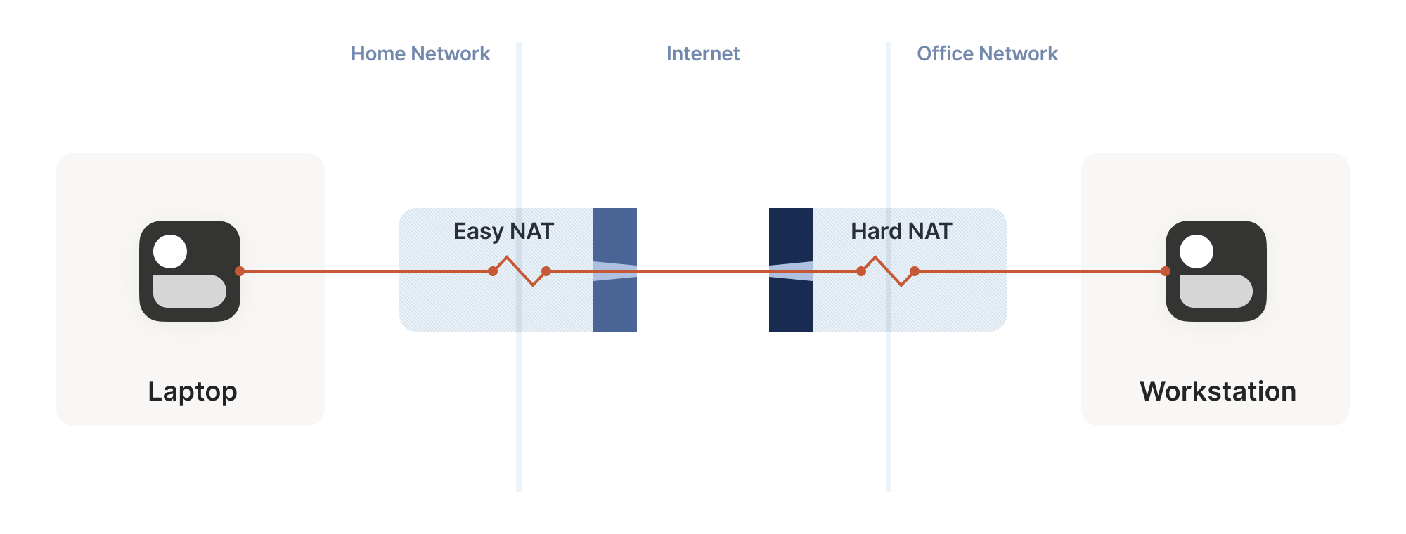
Well, we know some ip:port for the hard side, because we ran STUN. Let’s assume that the IP address we got is correct. That’s not necessarily true, but let’s run with the assumption for now. As it turns out, it’s mostly safe to assume this. (If you’re curious why, see REQ-2 in RFC 4787.)
If the IP address is correct, our only unknown is the port. There’s 65,535 possibilities… Could we try all of them? At 100 packets/sec, that’s a worst case of 10 minutes to find the right one. It’s better than nothing, but not great. And it really looks like a port scan (because in fairness, it is), which may anger network intrusion detection software.
We can do much better than that, with the help of the birthday paradox. Rather than open 1 port on the hard side and have the easy side try 65,535 possibilities, let’s open, say, 256 ports on the hard side (by having 256 sockets sending to the easy side’s ip:port), and have the easy side probe target ports at random.
I’ll spare you the detailed math, but you can check out the dinky python calculator I made while working it out. The calculation is a very slight variant on the “classic” birthday paradox, because it’s looking at collisions between two sets containing distinct elements, rather than collisions within a single set. Fortunately, the difference works out slightly in our favor! Here’s the chances of a collision of open ports (i.e. successful communication), as the number of random probes from the easy side increases, and assuming 256 ports on the hard side:
=========================   =========================
Number of random probes    Chance of success
=========================   =========================
174                         50%
256                         64%
1024                        98%
2048                        99.9%
=========================   =========================
If we stick with a fairly modest probing rate of 100 ports/sec, half the time we’ll get through in under 2 seconds. And even if we get unlucky, 20 seconds in we’re virtually guaranteed to have found a way in, after probing less than 4% of the total search space.
That’s great! With this additional trick, one hard NAT in the path is an annoying speedbump, but we can manage. What about two?
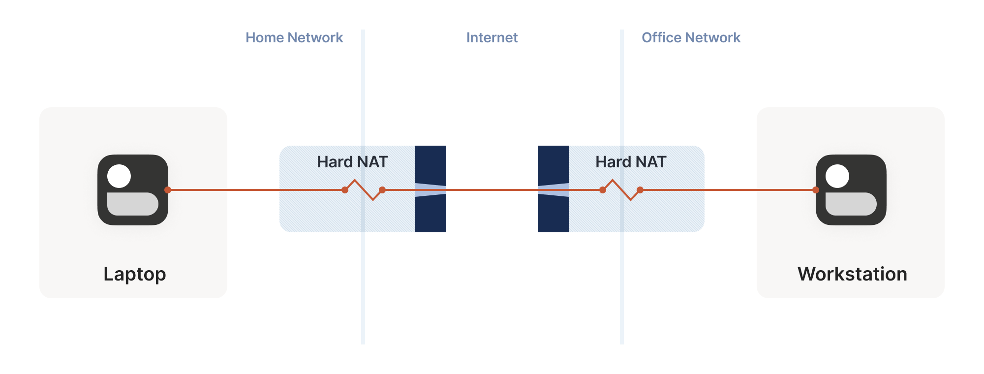
We can try to apply the same trick, but now the search is much harder: each random destination port we probe through a hard NAT also results in a random source port. That means we’re now looking for a collision on a {source port, destination port} pair, rather than just the destination port.
Again I’ll spare you the calculations, but after 20 seconds in the same regime as the previous setup (256 probes from one side, 2048 from the other), our chance of success is… 0.01%.
This shouldn’t be surprising if you’ve studied the birthday paradox before. The birthday paradox lets us convert N “effort” into something on the order of sqrt(N). But we squared the size of the search space, so even the reduced amount of effort is still a lot more effort. To hit a 99.9% chance of success, we need each side to send 170,000 probes. At 100 packets/sec, that’s 28 minutes of trying before we can communicate. 50% of the time we’ll succeed after “only” 54,000 packets, but that’s still 9 minutes of waiting around with no connection. Still, that’s better than the 1.2 years it would take without the birthday paradox.
In some applications, 28 minutes might still be worth it. Spend half an hour brute-forcing your way through, then you can keep pinging to keep the open path alive indefinitely — or at least until one of the NATs reboots and dumps all its state, then you’re back to brute forcing. But it’s not looking good for any kind of interactive connectivity.
Worse, if you look at common office routers, you’ll find that they have a surprisingly low limit on active sessions. For example, a Juniper SRX 300 maxes out at 64,000 active sessions. We’d consume its entire session table with our one attempt to get through! And that’s assuming the router behaves gracefully when overloaded. And this is all to get a single connection! What if we have 20 machines doing this behind the same router? Disaster.
Still, with this trick we can make it through a slightly harder network topology than before. That’s a big deal, because home routers tend to be easy NATs, and hard NATs tend to be office routers or cloud NAT gateways. That means this trick buys us improved connectivity for the home-to-office and home-to-cloud scenarios, as well as a few office-to-cloud and cloud-to-cloud scenarios.
Our hard NATs would be so much easier if we could ask the NATs to stop being such jerks, and let more stuff through. Turns out, there’s a protocol for that! Three of them, to be precise. Let’s talk about port mapping protocols.
The oldest is the UPnP IGD (Universal Plug’n’Play Internet Gateway Device) protocol. It was born in the late 1990’s, and as such uses a lot of very 90’s technology (XML, SOAP, multicast HTTP over UDP — yes, really) and is quite hard to implement correctly and securely — but a lot of routers shipped with UPnP, and a lot still do. If we strip away all the fluff, we find a very simple request-response that all three of our port mapping protocols implement: “Hi, please forward a WAN port to lan-ip:port,” and “okay, I’ve allocated wan-ip:port for you.”
Speaking of stripping away the fluff: some years after UPnP IGD came out, Apple launched a competing protocol called NAT-PMP (NAT Port Mapping Protocol). Unlike UPnP, it only does port forwarding, and is extremely simple to implement, both on clients and on NAT devices. A little bit after that, NAT-PMP v2 was reborn as PCP (Port Control Protocol).
So, to help our connectivity further, we can look for UPnP IGD, NAT-PMP and PCP on our local default gateway. If one of the protocols elicits a response, we request a public port mapping. You can think of this as a sort of supercharged STUN: in addition to discovering our public ip:port, we can instruct the NAT to be friendlier to our peers, by not enforcing firewall rules for that port. Any packet from anywhere that lands on our mapped port will make it back to us.
You can’t rely on these protocols being present. They might not be implemented on your devices. They might be disabled by default and nobody knew to turn them on. They might have been disabled by policy.
Disabling by policy is fairly common because UPnP suffered from a number of high-profile vulnerabilities (since fixed, so newer devices can safely offer UPnP, if implemented properly). Unfortunately, many devices come with a single “UPnP” checkbox that actually toggles UPnP, NAT-PMP and PCP all at once, so folks concerned about UPnP’s security end up disabling the perfectly safe alternatives as well.
Still, when it’s available, it effectively makes one NAT vanish from the data path, which usually makes connectivity trivial… But let’s look at the unusual cases.
So far, the topologies we’ve looked at have each client behind one NAT device, with the two NATs facing each other. What happens if we build a “double NAT”, by chaining two NATs in front of one of our machines?
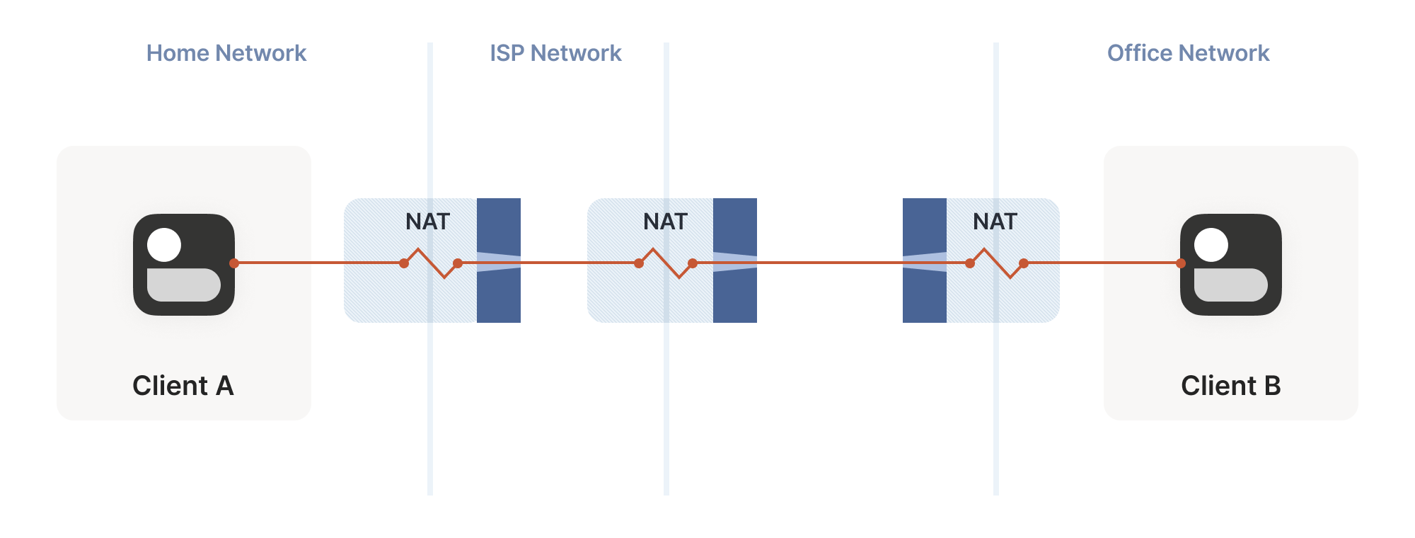
What happens if we build a “double NAT”, by chaining two NATs in front of one of our machines?
In this example, not much of interest happens. Packets from client A go through two different layers of NAT on their way to the internet. But the outcome is the same as it was with multiple layers of stateful firewalls: the extra layer is invisible to everyone, and our other techniques will work fine regardless of how many layers there are. All that matters is the behavior of the “last” layer before the internet, because that’s the one that our peer has to find a way through.
The big thing that breaks is our port mapping protocols. They act upon the layer of NAT closest to the client, whereas the one we need to influence is the one furthest away. You can still use the port mapping protocols, but you’ll get an ip:port in the “middle” network, which your remote peer cannot reach. Unfortunately, none of the protocols give you enough information to find the “next NAT up” to repeat the process there, although you could try your luck with a traceroute and some blind requests to the next few hops.
Breaking port mapping protocols is the reason why the internet is so full of warnings about the evils of double-NAT, and how you should bend over backwards to avoid them. But in fact, double-NAT is entirely invisible to most internet-using applications, because most applications don’t try to do this kind of explicit NAT traversal.
I’m definitely not saying that you should set up a double-NAT in your network. Breaking the port mapping protocols will degrade multiplayer on many video games, and will likely strip IPv6 from your network, which robs you of some very good options for NAT-free connectivity. But, if circumstances beyond your control force you into a double-NAT, and you can live with the downsides, most things will still work fine.
Which is a good thing, because you know what circumstances beyond your control force you to double-NAT? Let’s talk carrier-grade NAT.
Even with NATs to stretch the supply of IPv4 addresses, we’re still running out, and ISPs can no longer afford to give one entire public IP address to every home on their network. To work around this, ISPs apply SNAT recursively: your home router SNATs your devices to an “intermediate” IP address, and further out in the ISP’s network a second layer of NAT devices map those intermediate IPs onto a smaller number of public IPs. This is “carrier-grade NAT”, or CGNAT for short.
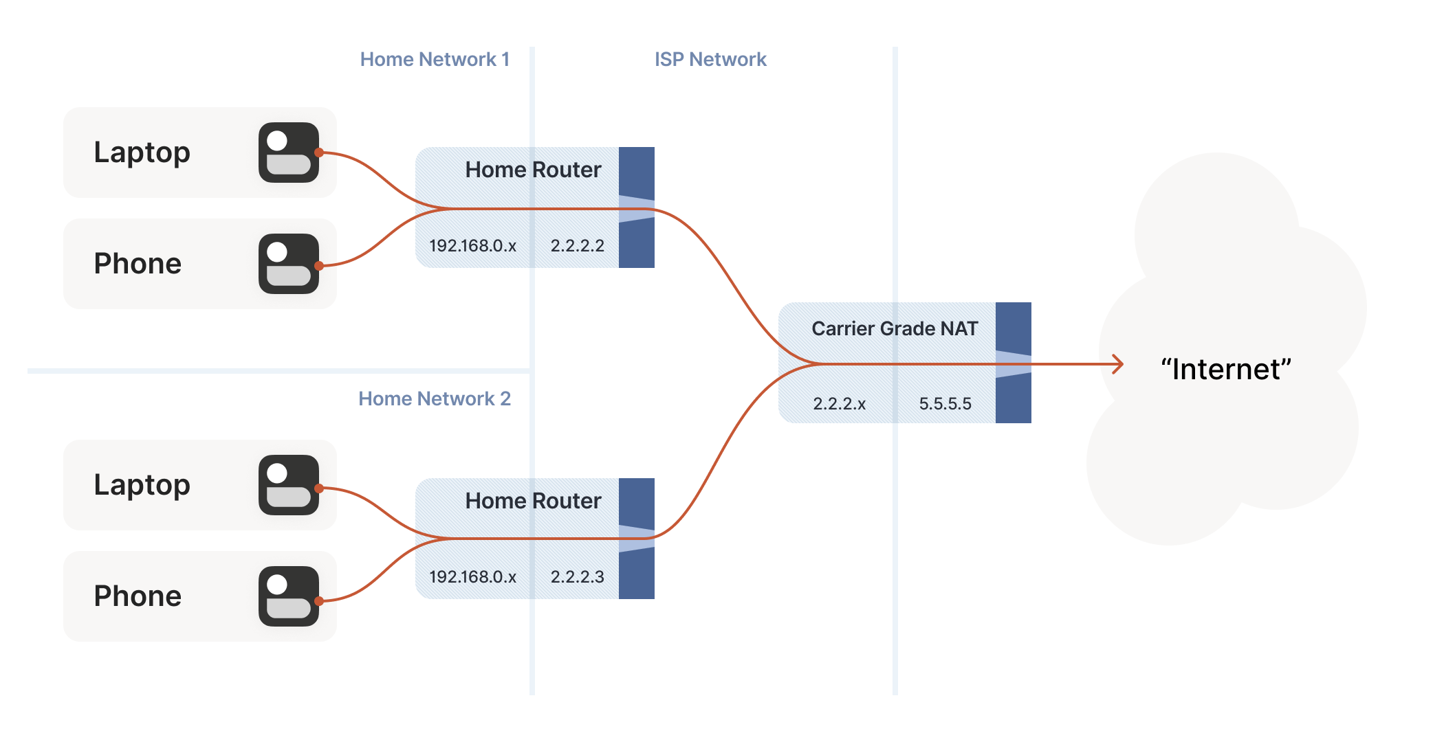
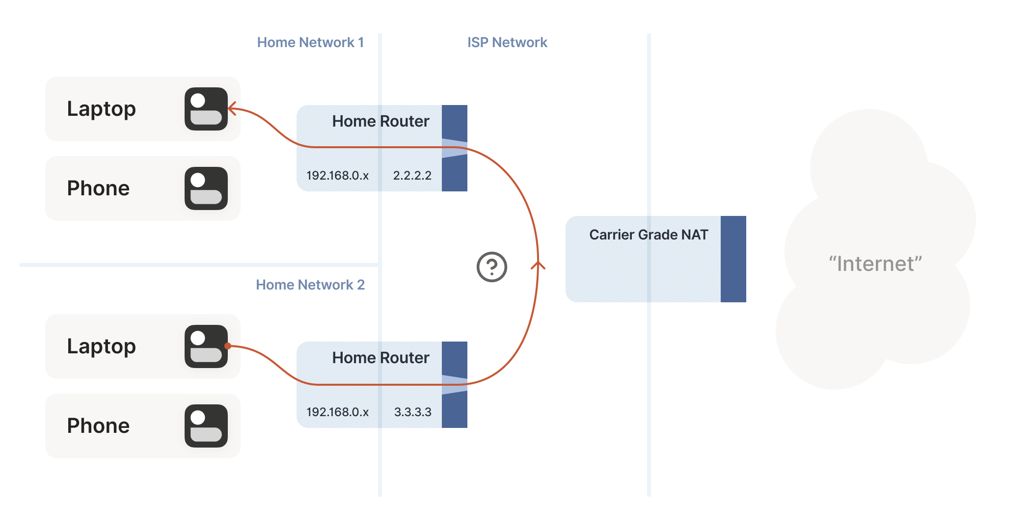
How do we connect two peers who are behind the same CGNAT, but different home NATs within?
Carrier-grade NAT is an important development for NAT traversal. Prior to CGNAT, enterprising users could work around NAT traversal difficulties by manually configuring port forwarding on their home routers. But you can’t reconfigure the ISP’s CGNAT! Now even power users have to wrestle with the problems NATs pose.
The good news: this is a run of the mill double-NAT, and so as we covered above it’s mostly okay. Some stuff won’t work as well as it could, but things work well enough that ISPs can charge money for it. Aside from the port mapping protocols, everything from our current bag of tricks works fine in a CGNAT world.
We do have to overcome a new challenge, however: how do we connect two peers who are behind the same CGNAT, but different home NATs within? That’s how we set up peers A and B in the diagram above.
The problem here is that STUN doesn’t work the way we’d like. We’d like to find out our ip:port on the “middle network”, because it’s effectively playing the role of a miniature internet to our two peers. But STUN tells us what our ip:port is from the STUN server’s point of view, and the STUN server is out on the internet, beyond the CGNAT.
If you’re thinking that port mapping protocols can help us here, you’re right! If either peer’s home NAT supports one of the port mapping protocols, we’re happy, because we have an ip:port that behaves like an un-NATed server, and connecting is trivial. Ironically, the fact that double NAT “breaks” the port mapping protocols helps us! Of course, we still can’t count on these protocols helping us out, doubly so because CGNAT ISPs tend to turn them off in the equipment they put in homes in order to avoid software getting confused by the “wrong” results they would get.
But what if we don’t get lucky, and can’t map ports on our NATs? Let’s go back to our STUN-based technique and see what happens. Both peers are behind the same CGNAT, so let’s say that STUN tells us that peer A is 2.2.2.2:1234, and peer B is 2.2.2.2:5678.
The question is: what happens when peer A sends a packet to 2.2.2.2:5678? We might hope that the following takes place in the CGNAT box:
-
Apply peer A’s NAT mapping, rewrite the packet to be from
2.2.2.2:1234and to2.2.2.2:5678. -
Notice that
2.2.2.2:5678matches peer B’s incoming NAT mapping, rewrite the packet to be from2.2.2.2:1234and to peer B’s private IP. -
Send the packet on to peer B, on the “internal” interface rather than off towards the internet.
This behavior of NATs is called hairpinning, and with all this dramatic buildup you won’t be surprised to learn that hairpinning works on some NATs and not others.
In fact, a great many otherwise well-behaved NAT devices don’t support hairpinning, because they make assumptions like “a packet from my internal network to a non-internal IP address will always flow outwards to the internet”, and so end up dropping packets as they try to turn around within the router. These assumptions might even be baked into routing silicon, where it’s impossible to fix without new hardware.
Hairpinning, or lack thereof, is a trait of all NATs, not just CGNATs. In most cases, it doesn’t matter, because you’d expect two LAN devices to talk directly to each other rather than hairpin through their default gateway. And it’s a pity that it usually doesn’t matter, because that’s probably why hairpinning is commonly broken.
But once CGNAT is involved, hairpinning becomes vital to connectivity. Hairpinning lets you apply the same tricks that you use for internet connectivity, without worrying about whether you’re behind a CGNAT. If both hairpinning and port mapping protocols fail, you’re stuck with relaying.
By this point I expect some of you are shouting at your screens that the solution to all this nonsense is IPv6. All this is happening because we’re running out of IPv4 addresses, and we keep piling on NATs to work around that. A much simpler fix would be to not have an IP address shortage, and make every device in the world reachable without NATs. Which is exactly what IPv6 gets us.
And you’re right! Sort of. It’s true that in an IPv6-only world, all of this becomes much simpler. Not trivial, mind you, because we’re still stuck with stateful firewalls. Your office workstation may have a globally reachable IPv6 address, but I’ll bet there’s still a corporate firewall enforcing “outbound connections only” between you and the greater internet. And on-device firewalls are still there, enforcing the same thing.
So, we still need the firewall traversal stuff from the start of the article, and a side channel so that peers can know what ip:port to talk to. We’ll probably also still want fallback relays that use a well-like protocol like HTTP, to get out of networks that block outbound UDP. But we can get rid of STUN, the birthday paradox trick, port mapping protocols, and all the hairpinning bumf. That’s much nicer!
The big catch is that we currently don’t have an all-IPv6 world. We have a world that’s mostly IPv4, and about 33% IPv6. Those 34% are very unevenly distributed, so a particular set of peers could be 100% IPv6, 0% IPv6, or anywhere in between.
What this means, unfortunately, is that IPv6 isn’t yet the solution to our problems. For now, it’s just an extra tool in our connectivity toolbox. It’ll work fantastically well with some pairs of peers, and not at all for others. If we’re aiming for “connectivity no matter what”, we have to also do IPv4+NAT stuff.
Meanwhile, the coexistence of IPv6 and IPv4 introduces yet another new scenario we have to account for: NAT64 devices.
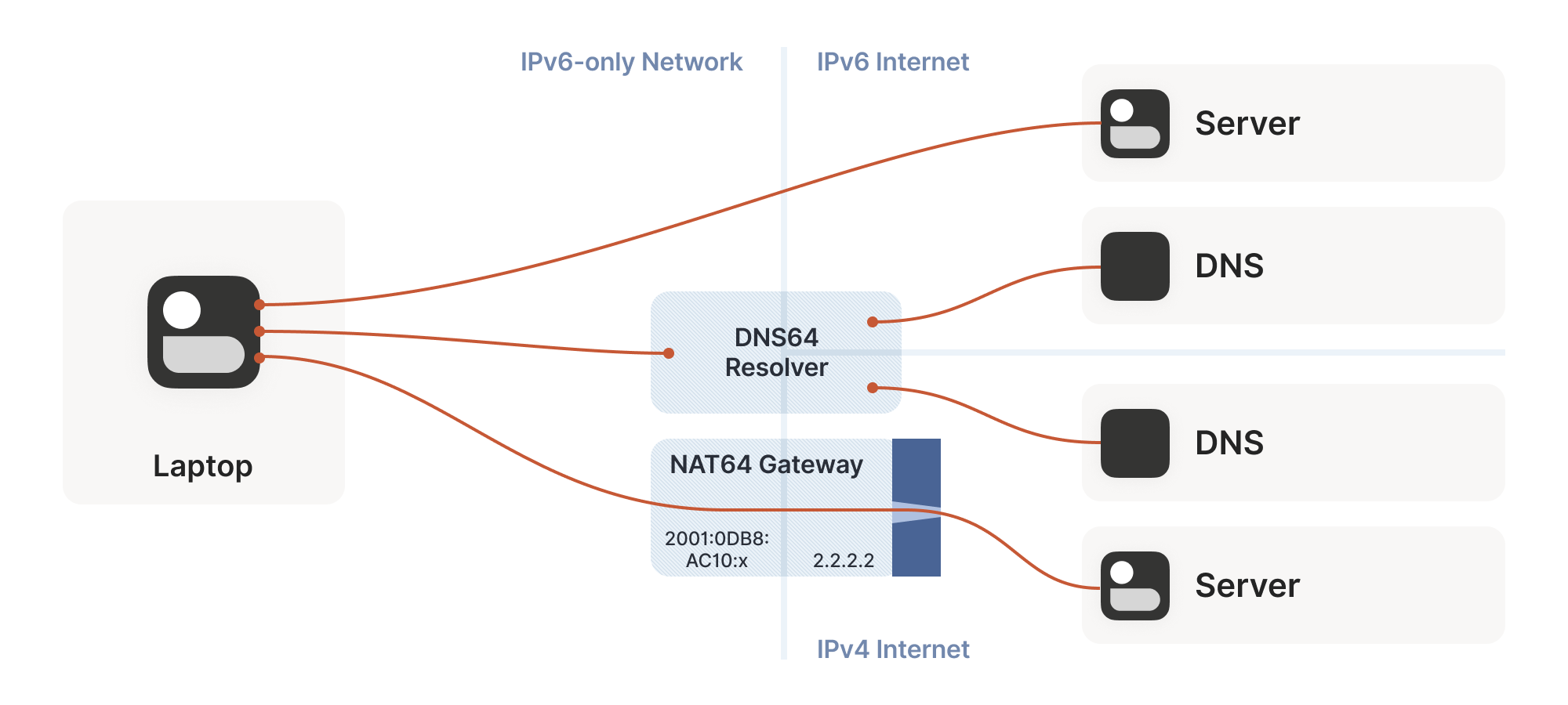
So far, the NATs we’ve looked at have been NAT44: they translate IPv4 addresses on one side to different IPv4 addresses on the other side. NAT64, as you might guess, translates between protocols. IPv6 on the internal side of the NAT becomes IPv4 on the external side. Combined with DNS64 to translate IPv4 DNS answers into IPv6, you can present an IPv6-only network to the end device, while still giving access to the IPv4 internet.
(Incidentally, you can extend this naming scheme indefinitely. There have been some experiments with NAT46; you could deploy NAT66 if you enjoy chaos; and some RFCs use NAT444 for carrier-grade NAT.)
This works fine if you only deal in DNS names. If you connect to google.com, turning that into an IP address involves the DNS64 apparatus, which lets the NAT64 get involved without you being any the wiser.
But we care deeply about specific IPs and ports for our NAT and firewall traversal. What about us? If we’re lucky, our device supports CLAT (Customer-side translator — from Customer XLAT). CLAT makes the OS pretend that it has direct IPv4 connectivity, using NAT64 behind the scenes to make it work out. On CLAT devices, we don’t need to do anything special.
CLAT is very common on mobile devices, but very uncommon on desktops, laptops and servers. On those, we have to explicitly do the work CLAT would have done: detect the existence of a NAT64+DNS64 setup, and use it appropriately.
Detecting NAT64+DNS64 is easy: send a DNS request to ipv4only.arpa. That name resolves to known, constant IPv4 addresses, and only IPv4 addresses. If you get IPv6 addresses back, you know that a DNS64 did some translation to steer you to a NAT64. That lets you figure out what the NAT64 prefix is.
From there, to talk to IPv4 addresses, send IPv6 packets to {NAT64 prefix + IPv4 address}. Similarly, if you receive traffic from {NAT64 prefix + IPv4 address}, that’s IPv4 traffic. Now speak STUN through the NAT64 to discover your public ip:port on the NAT64, and you’re back to the classic NAT traversal problem — albeit with a bit more work.
Fortunately for us, this is a fairly esoteric corner case. Most v6-only networks today are mobile operators, and almost all phones support CLAT. ISPs running v6-only networks deploy CLAT on the router they give you, and again you end up none the wiser. But if you want to get those last few opportunities for connectivity, you’ll have to explicitly support talking to v4-only peers from a v6-only network as well.
We’re in the home stretch. We’ve covered stateful firewalls, simple and advanced NAT tricks, IPv4 and IPv6. So, implement all the above, and we’re done!
Except, how do you figure out which tricks to use for a particular peer? How do you figure out if this is a simple stateful firewall problem, or if it’s time to bust out the birthday paradox, or if you need to fiddle with NAT64 by hand? Or maybe the two of you are on the same Wi-Fi network, with no firewalls and no effort required.
Early research into NAT traversal had you precisely characterize the path between you and your peer, and deploy a specific set of workarounds to defeat that exact path. But as it turned out, network engineers and NAT box programmers have many inventive ideas, and that stops scaling very quickly. We need something that involves a bit less thinking on our part.
Enter the Interactive Connectivity Establishment (ICE) protocol. Like STUN and TURN, ICE has its roots in the telephony world, and so the RFC is full of SIP and SDP and signalling sessions and dialing and so forth. However, if you push past that, it also specifies a stunningly elegant algorithm for figuring out the best way to get a connection.
Ready? The algorithm is: try everything at once, and pick the best thing that works. That’s it. Isn’t that amazing?
Let’s look at this algorithm in a bit more detail. We’re going to deviate from the ICE spec here and there, so if you’re trying to implement an interoperable ICE client, you should go read RFC 8445 and implement that. We’ll skip all the telephony-oriented stuff to focus on the core logic, and suggest a few places where you have more degrees of freedom than the ICE spec suggests.
To communicate with a peer, we start by gathering a list of candidate endpoints for our local socket. A candidate is any ip:port that our peer might, perhaps, be able to use in order to speak to us. We don’t need to be picky at this stage, the list should include at least:
-
IPv6
ip:ports -
IPv4 LAN
ip:ports -
IPv4 WAN
ip:portsdiscovered by STUN (possibly via a NAT64 translator) -
IPv4 WAN
ip:portallocated by a port mapping protocol -
Operator-provided endpoints (e.g. for statically configured port forwards)
Then, we swap candidate lists with our peer through the side channel, and start sending probe packets at each others’ endpoints. Again, at this point you don’t discriminate: if the peer provided you with 15 endpoints, you send “are you there?” probes to all 15 of them.
These packets are pulling double duty. Their first function is to act as the packets that open up the firewalls and pierce the NATs, like we’ve been doing for this entire article. But the other is to act as a health check. We’re exchanging (hopefully authenticated) “ping” and “pong” packets, to check if a particular path works end to end.
Finally, after some time has passed, we pick the “best” (according to some heuristic) candidate path that was observed to work, and we’re done.
The beauty of this algorithm is that if your heuristic is right, you’ll always get an optimal answer. ICE has you score your candidates ahead of time (usually: LAN > WAN > WAN+NAT), but it doesn’t have to be that way. Starting with v0.100.0, Tailscale switched from a hardcoded preference order to round-trip latency, which tends to result in the same LAN > WAN > WAN+NAT ordering. But unlike static ordering, we discover which “category” a path falls into organically, rather than having to guess ahead of time.
The ICE spec structures the protocol as a “probe phase” followed by an “okay let’s communicate” phase, but there’s no reason you need to strictly order them. In Tailscale, we upgrade connections on the fly as we discover better paths, and all connections start out with DERP preselected. That means you can use the connection immediately through the fallback path, while path discovery runs in parallel. Usually, after a few seconds, we’ll have found a better path, and your connection transparently upgrades to it.
One thing to be wary of is asymmetric paths. ICE goes to some effort to ensure that both peers have picked the same network path, so that there’s definite bidirectional packet flow to keep all the NATs and firewalls open. You don’t have to go to the same effort, but you do have to ensure that there’s bidirectional traffic along all paths you’re using. That can be as simple as continuing to send ping/pong probes periodically.
To be really robust, you also need to detect that your currently selected path has failed (say, because maintenance caused your NAT’s state to get dumped on the floor), and downgrade to another path. You can do this by continuing to probe all possible paths and keep a set of “warm” fallbacks ready to go, but downgrades are rare enough that it’s probably more efficient to fall all the way back to your relay of last resort, then restart path discovery.
Finally, we should mention security. Throughout this article, I’ve assumed that the “upper layer” protocol you’ll be running over this connection brings its own security (QUIC has TLS certs, WireGuard has its own public keys…). If that’s not the case, you absolutely need to bring your own. Once you’re dynamically switching paths at runtime, IP-based security becomes meaningless (not that it was worth much in the first place), and you must have at least end-to-end authentication.
If you have security for your upper layer, strictly speaking it’s okay if your ping/pong probes are spoofable. The worst that can happen is that an attacker can persuade you to relay your traffic through them. In the presence of e2e security, that’s not a huge deal (although obviously it depends on your threat model). But for good measure, you might as well authenticate and encrypt the path discovery packets as well. Consult your local application security engineer for how to do that safely.
At last, we’re done. If you implement all of the above, you’ll have state of the art NAT traversal software that can get direct connections established in the widest possible array of situations. And you’ll have your relay network to pick up the slack when traversal fails, as it likely will for a long tail of cases.
This is all quite complicated! It’s one of those problems that’s fun to explore, but quite fiddly to get right, especially if you start chasing the long tail of opportunities for just that little bit more connectivity.
The good news is that, once you’ve done it, you have something of a superpower: you get to explore the exciting and relatively under-explored world of peer-to-peer applications. So many interesting ideas for decentralized software fall at the first hurdle, when it turns out that talking to each other on the internet is harder than expected. But now you know how to get past that, so go build cool stuff!
Here’s a parting “TL;DR” recap: For robust NAT traversal, you need the following ingredients:
-
A UDP-based protocol to augment
-
Direct access to a socket in your program
-
A communication side channel with your peers
-
A couple of STUN servers
-
A network of fallback relays (optional, but highly recommended)
Then, you need to:
-
Enumerate all the
ip:portsfor your socket on your directly connected interfaces -
Query STUN servers to discover WAN
ip:portsand the “difficulty” of your NAT, if any -
Try using the port mapping protocols to find more WAN
ip:ports -
Check for NAT64 and discover a WAN
ip:portthrough that as well, if applicable -
Exchange all those
ip:portswith your peer through your side channel, along with some cryptographic keys to secure everything. -
Begin communicating with your peer through fallback relays (optional, for quick connection establishment)
-
Probe all of your peer’s
ip:portsfor connectivity and if necessary/desired, also execute birthday attacks to get through harder NATs -
As you discover connectivity paths that are better than the one you’re currently using, transparently upgrade away from the previous paths.
-
If the active path stops working, downgrade as needed to maintain connectivity.
-
Make sure everything is encrypted and authenticated end-to-end.
/Peer-to-Peer Communication Across Network Address Translators Ford, B., Srisuresh, P., and Kegel, D.
Bryan Ford
Massachusetts Institute of Technology
baford (at) mit.edu
Pyda Srisuresh
Caymas Systems, Inc.
srisuresh (at) yahoo.com
Dan Kegel
dank (at) kegel.com
J'fais des trous, des petits trous! ... toujours des petits trous
- S. Gainsbourg
Network Address Translation (NAT) causes well-known difficulties for peer-to-peer (P2P) communication, since the peers involved may not be reachable at any globally valid IP address. Several NAT traversal techniques are known, but their documentation is slim, and data about their robustness or relative merits is slimmer. This paper documents and analyzes one of the simplest but most robust and practical NAT traversal techniques, commonly known as “hole punching.” Hole punching is moderately well-understood for UDP communication, but we show how it can be reliably used to set up peer-to-peer TCP streams as well. After gathering data on the reliability of this technique on a wide variety of deployed NATs, we find that about 82% of the NATs tested support hole punching for UDP, and about 64% support hole punching for TCP streams. As NAT vendors become increasingly conscious of the needs of important P2P applications such as Voice over IP and online gaming protocols, support for hole punching is likely to increase in the future.
The combined pressures of tremendous growth and massive security challenges have forced the Internet to evolve in ways that make life difficult for many applications. The Internet's original uniform address architecture, in which every node has a globally unique IP address and can communicate directly with every other node, has been replaced with a new de facto Internet address architecture, consisting of a global address realm and many private address realms interconnected by Network Address Translators (NAT). In this new address architecture, illustrated in Figure [1], only nodes in the “main,” global address realm can be easily contacted from anywhere in the network, because only they have unique, globally routable IP addresses. Nodes on private networks can connect to other nodes on the same private network, and they can usually open TCP or UDP connections to “well-known” nodes in the global address realm. NATs on the path allocate temporary public endpoints for outgoing connections, and translate the addresses and port numbers in packets comprising those sessions, while generally blocking all incoming traffic unless otherwise specifically configured.
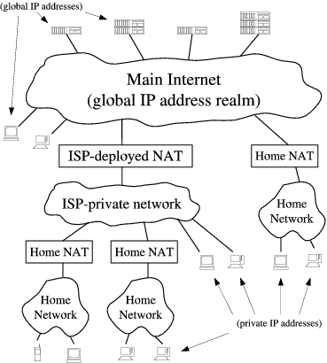
Figure 1: Public and private IP address domains
The Internet's new de facto address architecture is suitable for client/server communication in the typical case when the client is on a private network and the server is in the global address realm. The architecture makes it difficult for two nodes on different private networks to contact each other directly, however, which is often important to the “peer-to-peer” communication protocols used in applications such as teleconferencing and online gaming. We clearly need a way to make such protocols function smoothly in the presence of NAT.
One of the most effective methods of establishing peer-to-peer communication between hosts on different private networks is known as “hole punching.” This technique is widely used already in UDP-based applications, but essentially the same technique also works for TCP. Contrary to what its name may suggest, hole punching does not compromise the security of a private network. Instead, hole punching enables applications to function within the the default security policy of most NATs, effectively signaling to NATs on the path that peer-to-peer communication sessions are “solicited” and thus should be accepted. This paper documents hole punching for both UDP and TCP, and details the crucial aspects of both application and NAT behavior that make hole punching work.
Unfortunately, no traversal technique works with all existing NATs, because NAT behavior is not standardized. This paper presents some experimental results evaluating hole punching support in current NATs. Our data is derived from results submitted by users throughout the Internet by running our “NAT Check” tool over a wide variety of NATs by different vendors. While the data points were gathered from a “self-selecting” user community and may not be representative of the true distribution of NAT implementations deployed on the Internet, the results are nevertheless generally encouraging.
While evaluating basic hole punching, we also point out variations that can make hole punching work on a wider variety of existing NATs at the cost of greater complexity. Our primary focus, however, is on developing the simplest hole punching technique that works cleanly and robustly in the presence of “well-behaved” NATs in any reasonable network topology. We deliberately avoid excessively clever tricks that may increase compatibility with some existing “broken” NATs in the short term, but which only work some of the time and may cause additional unpredictability and network brittleness in the long term.
Although the larger address space of IPv6 [3] may eventually reduce the need for NAT, in the short term IPv6 is increasing the demand for NAT, because NAT itself provides the easiest way to achieve interoperability between IPv4 and IPv6 address domains [24]. Further, the anonymity and inaccessibility of hosts on private networks has widely perceived security and privacy benefits. Firewalls are unlikely to go away even when there are enough IP addresses: IPv6 firewalls will still commonly block unsolicited incoming traffic by default, making hole punching useful even to IPv6 applications.
The rest of this paper is organized as follows. Section [2] introduces basic terminology and NAT traversal concepts. Section [3] details hole punching for UDP, and Section [4] introduces hole punching for TCP. Section [5] summarizes important properties a NAT must have in order to enable hole punching. Section [6] presents our experimental results on hole punching support in popular NATs, Section [7] discusses related work, and Section [8] concludes.
This section introduces basic NAT terminology used throughout the paper, and then outlines general NAT traversal techniques that apply equally to TCP and UDP.
This paper adopts the NAT terminology and taxonomy defined in RFC 2663 [21], as well as additional terms defined more recently in RFC 3489 [19].
Of particular importance is the notion of session. A session endpoint for TCP or UDP is an (IP address, port number) pair, and a particular session is uniquely identified by its two session endpoints. From the perspective of one of the hosts involved, a session is effectively identified by the 4-tuple (local IP, local port, remote IP, remote port). The direction of a session is normally the flow direction of the packet that initiates the session: the initial SYN packet for TCP, or the first user datagram for UDP.
Of the various flavors of NAT, the most common type is traditional or outbound NAT, which provides an asymmetric bridge between a private network and a public network. Outbound NAT by default allows only outbound sessions to traverse the NAT: incoming packets are dropped unless the NAT identifies them as being part of an existing session initiated from within the private network. Outbound NAT conflicts with peer-to-peer protocols because when both peers desiring to communicate are “behind” (on the private network side of) two different NATs, whichever peer tries to initiate a session, the other peer's NAT rejects it. NAT traversal entails making P2P sessions look like “outbound” sessions to both NATs.
Outbound NAT has two sub-varieties: Basic NAT, which only translates IP addresses, and Network Address/Port Translation (NAPT), which translates entire session endpoints. NAPT, the more general variety, has also become the most common because it enables the hosts on a private network to share the use of a single public IP address. Throughout this paper we assume NAPT, though the principles and techniques we discuss apply equally well (if sometimes trivially) to Basic NAT.
The most reliable--but least efficient--method of P2P communication across NAT is simply to make the communication look to the network like standard client/server communication, through relaying. Suppose two client hosts 𝓐 and 𝓑 have each initiated TCP or UDP connections to a well-known server 𝓢, at 𝓢's global IP address 18.181.0.31 and port number 1234. As shown in Figure 2, the clients reside on separate private networks, and their respective NATs prevent either client from directly initiating a connection to the other. Instead of attempting a direct connection, the two clients can simply use the server 𝓢 to relay messages between them. For example, to send a message to client 𝓑, client 𝓐 simply sends the message to server 𝓢 along its already-established client/server connection, and server 𝓢 forwards the message on to client 𝓑 using its existing client/server connection with 𝓑.
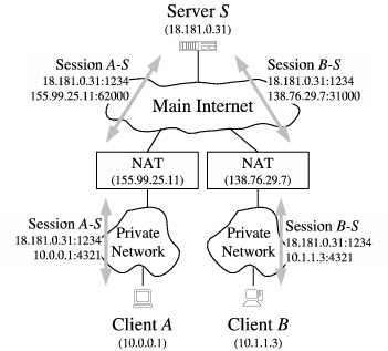
Figure 2: NAT Traversal by Relaying
Relaying always works as long as both clients can connect to the server. Its disadvantages are that it consumes the server's processing power and network bandwidth, and communication latency between the peering clients is likely increased even if the server is well-connected. Nevertheless, since there is no more efficient technique that works reliably on all existing NATs, relaying is a useful fall-back strategy if maximum robustness is desired. The TURN protocol [18] defines a method of implementing relaying in a relatively secure fashion.
Some P2P applications use a straightforward but limited technique, known as connection reversal, to enable communication when both hosts have connections to a well-known rendezvous server 𝓢 and only one of the peers is behind a NAT, as shown in Figure 3. If 𝓐 wants to initiate a connection to 𝓑, then a direct connection attempt works automatically, because 𝓑 is not behind a NAT and 𝓐's NAT interprets the connection as an outgoing session. If 𝓑 wants to initiate a connection to 𝓐, however, any direct connection attempt to 𝓐 is blocked by 𝓐's NAT. 𝓑 can instead relay a connection request to 𝓐 through a well-known server 𝓢, asking 𝓐 to attempt a “reverse” connection back to 𝓑. Despite the obvious limitations of this technique, the central idea of using a well-known rendezvous server as an intermediary to help set up direct peer-to-peer connections is fundamental to the more general hole punching techniques described next.
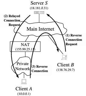
Figure 3: NAT Traversal by Connection Reversal
UDP hole punching enables two clients to set up a direct peer-to-peer UDP session with the help of a well-known rendezvous server, even if the clients are both behind NATs. This technique was mentioned in section 5.1 of RFC 3027 [10], documented more thoroughly elsewhere on the Web [13], and used in recent experimental Internet protocols [17,11]. Various proprietary protocols, such as those for on-line gaming, also use UDP hole punching.
Hole punching assumes that the two clients, 𝓐 and 𝓑, already have active UDP sessions with a rendezvous server 𝓢. When a client registers with 𝓢, the server records two endpoints for that client: the (IP address, UDP port) pair that the client believes itself to be using to talk with 𝓢, and the (IP address, UDP port) pair that the server observes the client to be using to talk with it. We refer to the first pair as the client's private endpoint and the second as the client's public endpoint. The server might obtain the client's private endpoint from the client itself in a field in the body of the client's registration message, and obtain the client's public endpoint from the source IP address and source UDP port fields in the IP and UDP headers of that registration message. If the client is not behind a NAT, then its private and public endpoints should be identical.
A few poorly behaved NATs are known to scan the body of UDP datagrams for 4-byte fields that look like IP addresses, and translate them as they would the IP address fields in the IP header. To be robust against such behavior, applications may wish to obfuscate IP addresses in messages bodies slightly, for example by transmitting the one's complement of the IP address instead of the IP address itself. Of course, if the application is encrypting its messages, then this behavior is not likely to be a problem.
Suppose client 𝓐 wants to establish a UDP session directly with client 𝓑. Hole punching proceeds as follows:
-
𝓐 initially does not know how to reach 𝓑, so 𝓐 asks 𝓢 for help establishing a UDP session with 𝓑.
-
𝓢 replies to 𝓐 with a message containing 𝓑's public and private endpoints. At the same time, 𝓢 uses its UDP session with 𝓑 to send 𝓑 a connection request message containing 𝓐's public and private endpoints. Once these messages are received, 𝓐 and 𝓑 know each other's public and private endpoints.
-
When 𝓐 receives 𝓑's public and private endpoints from 𝓢, 𝓐 starts sending UDP packets to both of these endpoints, and subsequently “locks in” whichever endpoint first elicits a valid response from 𝓑. Similarly, when 𝓑 receives 𝓐's public and private endpoints in the forwarded connection request, 𝓑 starts sending UDP packets to 𝓐 at each of 𝓐's known endpoints, locking in the first endpoint that works. The order and timing of these messages are not critical as long as they are asynchronous.
We now consider how UDP hole punching handles each of three specific network scenarios. In the first situation, representing the “easy” case, the two clients actually reside behind the same NAT, on one private network. In the second, most common case, the clients reside behind different NATs. In the third scenario, the clients each reside behind two levels of NAT: a common “first-level” NAT deployed by an ISP for example, and distinct “second-level” NATs such as consumer NAT routers for home networks.
It is in general difficult or impossible for the application itself to determine the exact physical layout of the network, and thus which of these scenarios (or the many other possible ones) actually applies at a given time. Protocols such as STUN [19] can provide some information about the NATs present on a communication path, but this information may not always be complete or reliable, especially when multiple levels of NAT are involved. Nevertheless, hole punching works automatically in all of these scenarios without the application having to know the specific network organization, as long as the NATs involved behave in a reasonable fashion. (“Reasonable” behavior for NATs will be described later in Section [5].)
First consider the simple scenario in which the two clients (probably unknowingly) happen to reside behind the same NAT, and are therefore located in the same private IP address realm, as shown in Figure 4. Client 𝓐 has established a UDP session with server 𝓢, to which the common NAT has assigned its own public port number 62000. Client 𝓑 has similarly established a session with 𝓢, to which the NAT has assigned public port number 62005.
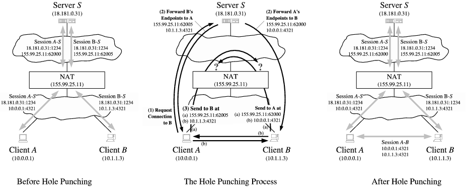
Figure 4: UDP Hole Punching, Peers Behind a Common NAT
Suppose that client 𝓐 uses the hole punching technique outlined above to establish a UDP session with 𝓑, using server 𝓢 as an introducer. Client 𝓐 sends 𝓢 a message requesting a connection to 𝓑. 𝓢 responds to 𝓐 with 𝓑's public and private endpoints, and also forwards 𝓐's public and private endpoints to 𝓑. Both clients then attempt to send UDP datagrams to each other directly at each of these endpoints. The messages directed to the public endpoints may or may not reach their destination, depending on whether or not the NAT supports hairpin translation as described below in Section [3.5]. The messages directed at the private endpoints do reach their destinations, however, and since this direct route through the private network is likely to be faster than an indirect route through the NAT anyway, the clients are most likely to select the private endpoints for subsequent regular communication.
By assuming that NATs support hairpin translation, the application might dispense with the complexity of trying private as well as public endpoints, at the cost of making local communication behind a common NAT unnecessarily pass through the NAT. As our results in Section [6] show, however, hairpin translation is still much less common among existing NATs than are other “P2P-friendly” NAT behaviors. For now, therefore, applications may benefit substantially by using both public and private endpoints.
Suppose clients 𝓐 and 𝓑 have private IP addresses behind different NATs, as shown in Figure 5. 𝓐 and 𝓑 have each initiated UDP communication sessions from their local port 4321 to port 1234 on server 𝓢. In handling these outbound sessions, NAT 𝓐 has assigned port 62000 at its own public IP address, 155.99.25.11, for the use of 𝓐's session with 𝓢, and NAT 𝓑 has assigned port 31000 at its IP address, 138.76.29.7, to 𝓑's session with 𝓢.
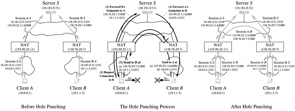
Figure 5: UDP Hole Punching, Peers Behind Different NATs
In 𝓐's registration message to 𝓢, 𝓐 reports its private endpoint to 𝓢 as 10.0.0.1:4321, where 10.0.0.1 is 𝓐's IP address on its own private network. 𝓢 records 𝓐's reported private endpoint, along with 𝓐's public endpoint as observed by 𝓢 itself. 𝓐's public endpoint in this case is 155.99.25.11:62000, the temporary endpoint assigned to the session by the NAT. Similarly, when client 𝓑 registers, 𝓢 records 𝓑's private endpoint as 10.1.1.3:4321 and 𝓑's public endpoint as 138.76.29.7:31000.
Now client 𝓐 follows the hole punching procedure described above to establish a UDP communication session directly with 𝓑. First, 𝓐 sends a request message to 𝓢 asking for help connecting with 𝓑. In response, 𝓢 sends 𝓑's public and private endpoints to 𝓐, and sends 𝓐's public and private endpoints to 𝓑. 𝓐 and 𝓑 each start trying to send UDP datagrams directly to each of these endpoints.
Since 𝓐 and 𝓑 are on different private networks and their respective private IP addresses are not globally routable, the messages sent to these endpoints will reach either the wrong host or no host at all. Because many NATs also act as DHCP servers, handing out IP addresses in a fairly deterministic way from a private address pool usually determined by the NAT vendor by default, it is quite likely in practice that 𝓐's messages directed at 𝓑's private endpoint will reach some (incorrect) host on 𝓐's private network that happens to have the same private IP address as 𝓑 does. Applications must therefore authenticate all messages in some way to filter out such stray traffic robustly. The messages might include application-specific names or cryptographic tokens, for example, or at least a random nonce pre-arranged through 𝓢.
Now consider 𝓐's first message sent to 𝓑's public endpoint, as shown in Figure 5. As this outbound message passes through 𝓐's NAT, this NAT notices that this is the first UDP packet in a new outgoing session. The new session's source endpoint (10.0.0.1:4321) is the same as that of the existing session between 𝓐 and 𝓢, but its destination endpoint is different. If NAT 𝓐 is well-behaved, it preserves the identity of 𝓐's private endpoint, consistently translating all outbound sessions from private source endpoint 10.0.0.1:4321 to the corresponding public source endpoint 155.99.25.11:62000. 𝓐's first outgoing message to 𝓑's public endpoint thus, in effect, “punches a hole” in 𝓐's NAT for a new UDP session identified by the endpoints (10.0.0.1:4321, 138.76.29.7:31000) on 𝓐's private network, and by the endpoints (155.99.25.11:62000, 138.76.29.7:31000) on the main Internet.
If 𝓐's message to 𝓑's public endpoint reaches 𝓑's NAT before 𝓑's first message to 𝓐 has crossed 𝓑's own NAT, then 𝓑's NAT may interpret 𝓐's inbound message as unsolicited incoming traffic and drop it. 𝓑's first message to 𝓐's public address, however, similarly opens a hole in 𝓑's NAT, for a new UDP session identified by the endpoints (10.1.1.3:4321, 155.99.25.11:62000) on 𝓑's private network, and by the endpoints (138.76.29.7:31000, 155.99.25.11:62000) on the Internet. Once the first messages from 𝓐 and 𝓑 have crossed their respective NATs, holes are open in each direction and UDP communication can proceed normally. Once the clients have verified that the public endpoints work, they can stop sending messages to the alternative private endpoints.
In some topologies involving multiple NAT devices, two clients cannot establish an “optimal” P2P route between them without specific knowledge of the topology. Consider a final scenario, depicted in Figure 6. Suppose NAT 𝓒 is a large industrial NAT deployed by an internet service provider (ISP) to multiplex many customers onto a few public IP addresses, and NATs 𝓐 and 𝓑 are small consumer NAT routers deployed independently by two of the ISP's customers to multiplex their private home networks onto their respective ISP-provided IP addresses. Only server 𝓢 and NAT 𝓒 have globally routable IP addresses; the “public” IP addresses used by NAT 𝓐 and NAT 𝓑 are actually private to the ISP's address realm, while client 𝓐's and 𝓑's addresses in turn are private to the addressing realms of NAT 𝓐 and NAT 𝓑, respectively. Each client initiates an outgoing connection to server 𝓢 as before, causing NATs 𝓐 and 𝓑 each to create a single public/private translation, and causing NAT 𝓒 to establish a public/private translation for each session.
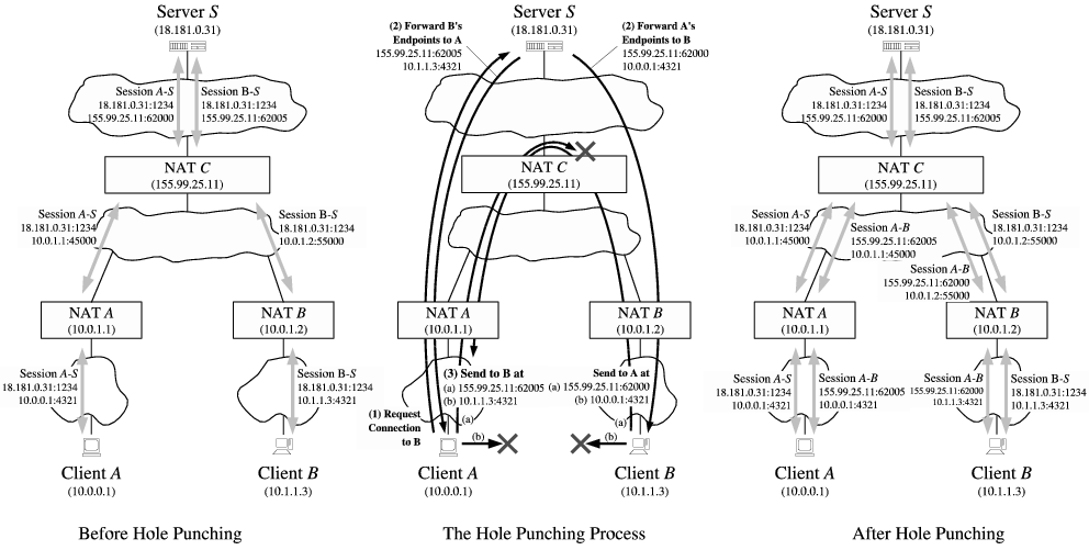
Figure 6: UDP Hole Punching, Peers Behind Multiple Levels of NAT
Now suppose 𝓐 and 𝓑 attempt to establish a direct peer-to-peer UDP connection via hole punching. The optimal routing strategy would be for client 𝓐 to send messages to client 𝓑's “semi-public” endpoint at NAT 𝓑, 10.0.1.2:55000 in the ISP's addressing realm, and for client 𝓑 to send messages to 𝓐's “semi-public” endpoint at NAT 𝓑, namely 10.0.1.1:45000. Unfortunately, 𝓐 and 𝓑 have no way to learn these addresses, because server 𝓢 only sees the truly global public endpoints of the clients, 155.99.25.11:62000 and 155.99.25.11:62005 respectively. Even if 𝓐 and 𝓑 had some way to learn these addresses, there is still no guarantee that they would be usable, because the address assignments in the ISP's private address realm might conflict with unrelated address assignments in the clients' private realms. (NAT 𝓐's IP address in NAT 𝓒's realm might just as easily have been 10.1.1.3, for example, the same as client 𝓑's private address in NAT 𝓑's realm.)
The clients therefore have no choice but to use their global public addresses as seen by 𝓢 for their P2P communication, and rely on NAT 𝓒 providing hairpin or loopback translation. When 𝓐 sends a UDP datagram to 𝓑's global endpoint, 155.99.25.11:62005, NAT 𝓐 first translates the datagram's source endpoint from 10.0.0.1:4321 to 10.0.1.1:45000. The datagram now reaches NAT 𝓒, which recognizes that the datagram's destination address is one of NAT 𝓒's own translated public endpoints. If NAT 𝓒 is well-behaved, it then translates both the source and destination addresses in the datagram and “loops” the datagram back onto the private network, now with a source endpoint of 155.99.25.11:62000 and a destination endpoint of 10.0.1.2:55000. NAT 𝓑 finally translates the datagram's destination address as the datagram enters 𝓑's private network, and the datagram reaches 𝓑. The path back to 𝓐 works similarly. Many NATs do not yet support hairpin translation, but it is becoming more common as NAT vendors become aware of this issue.
Since the UDP transport protocol provides NATs with no reliable, application-independent way to determine the lifetime of a session crossing the NAT, most NATs simply associate an idle timer with UDP translations, closing the hole if no traffic has used it for some time period. There is unfortunately no standard value for this timer: some NATs have timeouts as short as 20 seconds. If the application needs to keep an idle UDP session active after establishing the session via hole punching, the application must send periodic keep-alive packets to ensure that the relevant translation state in the NATs does not disappear.
Unfortunately, many NATs associate UDP idle timers with individual UDP sessions defined by a particular pair of endpoints, so sending keep-alives on one session will not keep other sessions active even if all the sessions originate from the same private endpoint. Instead of sending keep-alives on many different P2P sessions, applications can avoid excessive keep-alive traffic by detecting when a UDP session no longer works, and re-running the original hole punching procedure again “on demand.”
Establishing peer-to-peer TCP connections between hosts behind NATs is slightly more complex than for UDP, but TCP hole punching is remarkably similar at the protocol level. Since it is not as well-understood, it is currently supported by fewer existing NATs. When the NATs involved do support it, however, TCP hole punching is just as fast and reliable as UDP hole punching. Peer-to-peer TCP communication across well-behaved NATs may in fact be more robust than UDP communication, because unlike UDP, the TCP protocol's state machine gives NATs on the path a standard way to determine the precise lifetime of a particular TCP session.
The main practical challenge to applications wishing to implement TCP hole punching is not a protocol issue but an application programming interface (API) issue. Because the standard Berkeley sockets API was designed around the client/server paradigm, the API allows a TCP stream socket to be used to initiate an outgoing connection via connect(), or to listen for incoming connections via listen() and accept(), but not both. Further, TCP sockets usually have a one-to-one correspondence to TCP port numbers on the local host: after the application binds one socket to a particular local TCP port, attempts to bind a second socket to the same TCP port fail.
For TCP hole punching to work, however, we need to use a single local TCP port to listen for incoming TCP connections and to initiate multiple outgoing TCP connections concurrently. Fortunately, all major operating systems support a special TCP socket option, commonly named SO_REUSEADDR, which allows the application to bind multiple sockets to the same local endpoint as long as this option is set on all of the sockets involved. BSD systems have introduced a SO_REUSEPORT option that controls port reuse separately from address reuse; on such systems both of these options must be set.
Suppose that client 𝓐 wishes to set up a TCP connection with client 𝓑. We assume as usual that both 𝓐 and 𝓑 already have active TCP connections with a well-known rendezvous server 𝓢. The server records each registered client's public and private endpoints, just as for UDP. At the protocol level, TCP hole punching works almost exactly as for UDP:
-
Client 𝓐 uses its active TCP session with 𝓢 to ask 𝓢 for help connecting to 𝓑.
-
𝓢 replies to 𝓐 with 𝓑's public and private TCP endpoints, and at the same time sends 𝓐's public and private endpoints to 𝓑.
-
From the same local TCP ports that 𝓐 and 𝓑 used to register with 𝓢, 𝓐 and 𝓑 each asynchronously make outgoing connection attempts to the other's public and private endpoints as reported by 𝓢, while simultaneously listening for incoming connections on their respective local TCP ports.
-
𝓐 and 𝓑 wait for outgoing connection attempts to succeed, and/or for incoming connections to appear. If one of the outgoing connection attempts fails due to a network error such as “connection reset” or “host unreachable,” the host simply re-tries that connection attempt after a short delay (e.g., one second), up to an application-defind maximum timeout period.
-
When a TCP connection is made, the hosts authenticate each other to verify that they connected to the intended host. If authentication fails, the clients close that connection and continue waiting for others to succeed. The clients use the first successfully authenticated TCP stream resulting from this process.
Unlike with UDP, where each client only needs one socket to communicate with both 𝓢 and any number of peers simultaneously, with TCP each client application must manage several sockets bound to a single local TCP port on that client node, as shown in Figure 7. Each client needs a stream socket representing its connection to 𝓢, a listen socket on which to accept incoming connections from peers, and at least two additional stream sockets with which to initiate outgoing connections to the other peer's public and private TCP endpoints.
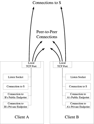
Figure 7: Sockets versus Ports for TCP Hole Punching
Consider the common-case scenario in which the clients 𝓐 and 𝓑 are behind different NATs, as shown in Figure 5, and assume that the port numbers shown in the figure are now for TCP rather than UDP ports. The outgoing connection attempts 𝓐 and 𝓑 make to each other's private endpoints either fail or connect to the wrong host. As with UDP, it is important that TCP applications authenticate their peer-to-peer sessions, due of the likelihood of mistakenly connecting to a random host on the local network that happens to have the same private IP address as the desired host on a remote private network.
The clients' outgoing connection attempts to each other's public endpoints, however, cause the respective NATs to open up new “holes” enabling direct TCP communication between 𝓐 and 𝓑. If the NATs are well-behaved, then a new peer-to-peer TCP stream automatically forms between them. If 𝓐's first SYN packet to 𝓑 reaches 𝓑's NAT before 𝓑's first SYN packet to 𝓐 reaches 𝓑's NAT, for example, then 𝓑's NAT may interpret 𝓐's SYN as an unsolicited incoming connection attempt and drop it. 𝓑's first SYN packet to 𝓐 should subsequently get through, however, because 𝓐's NAT sees this SYN as being part of the outbound session to 𝓑 that 𝓐's first SYN had already initiated.
What the client applications observe to happen with their sockets during TCP hole punching depends on the timing and the TCP implementations involved. Suppose that 𝓐's first outbound SYN packet to 𝓑's public endpoint is dropped by NAT 𝓑, but 𝓑's first subsequent SYN packet to 𝓐's public endpoint gets through to 𝓐 before 𝓐's TCP retransmits its SYN. Depending on the operating system involved, one of two things may happen:
-
𝓐's TCP implementation notices that the session endpoints for the incoming SYN match those of an outbound session 𝓐 was attempting to initiate. 𝓐's TCP stack therefore associates this new session with the socket that the local application on 𝓐 was using to connect() to 𝓑's public endpoint. The application's asynchronous connect() call succeeds, and nothing happens with the application's listen socket.
Since the received SYN packet did not include an ACK for 𝓐's previous outbound SYN, 𝓐's TCP replies to 𝓑's public endpoint with a SYN-ACK packet, the SYN part being merely a replay of 𝓐's original outbound SYN, using the same sequence number. Once 𝓑's TCP receives 𝓐's SYN-ACK, it responds with its own ACK for 𝓐's SYN, and the TCP session enters the connected state on both ends.
-
Alternatively, 𝓐's TCP implementation might instead notice that 𝓐 has an active listen socket on that port waiting for incoming connection attempts. Since 𝓑's SYN looks like an incoming connection attempt, 𝓐's TCP creates a new stream socket with which to associate the new TCP session, and hands this new socket to the application via the application's next accept() call on its listen socket. 𝓐's TCP then responds to 𝓑 with a SYN-ACK as above, and TCP connection setup proceeds as usual for client/server-style connections.
Since 𝓐's prior outbound connect() attempt to 𝓑 used a combination of source and destination endpoints that is now in use by another socket, namely the one just returned to the application via accept(), 𝓐's asynchronous connect() attempt must fail at some point, typically with an “address in use” error. The application nevertheless has the working peer-to-peer stream socket it needs to communicate with 𝓑, so it ignores this failure.
The first behavior above appears to be usual for BSD-based operating systems, whereas the second behavior appears more common under Linux and Windows.
Suppose that the timing of the various connection attempts during the hole punching process works out so that the initial outgoing SYN packets from both clients traverse their respective local NATs, opening new outbound TCP sessions in each NAT, before reaching the remote NAT. In this “lucky” case, the NATs do not reject either of the initial SYN packets, and the SYNs cross on the wire between the two NATs. In this case, the clients observe an event known as a simultaneous TCP open: each peer's TCP receives a “raw” SYN while waiting for a SYN-ACK. Each peer's TCP responds with a SYN-ACK, whose SYN part essentially “replays” the peer's previous outgoing SYN, and whose ACK part acknowledges the SYN received from the other peer.
What the respective applications observe in this case again depends on the behavior of the TCP implementations involved, as described in the previous section. If both clients implement the second behavior above, it may be that all of the asynchronous connect() calls made by the application ultimately fail, but the application running on each client nevertheless receives a new, working peer-to-peer TCP stream socket via accept()--as if this TCP stream had magically “created itself” on the wire and was merely passively accepted at the endpoints! As long as the application does not care whether it ultimately receives its peer-to-peer TCP sockets via connect() or accept(), the process results in a working stream on any TCP implementation that properly implements the standard TCP state machine specified in RFC 793 [23].
Each of the alternative network organization scenarios discussed in Section [3] for UDP works in exactly the same way for TCP. For example, TCP hole punching works in multi-level NAT scenarios such as the one in Figure 6 as long as the NATs involved are well-behaved.
In a variant of the above TCP hole punching procedure implemented by the NatTrav library [4], the clients attempt connections to each other sequentially rather than in parallel. For example: (1) 𝓐 informs 𝓑 via 𝓢 of its desire to communicate, without simultaneously listening on its local port; (2) 𝓑 makes a connect() attempt to 𝓐, which opens a hole in 𝓑's NAT but then fails due to a timeout or RST from 𝓐's NAT or a RST from 𝓐 itself; (3) 𝓑 closes its connection to 𝓢 and does a listen() on its local port; (4) 𝓢 in turn closes its connection with 𝓐, signaling 𝓐 to attempt a connect() directly to 𝓑.
This sequential procedure may be particularly useful on Windows hosts prior to XP Service Pack 2, which did not correctly implement simultaneous TCP open, or on sockets APIs that do not support the SO_REUSEADDR functionality. The sequential procedure is more timing-dependent, however, and may be slower in the common case and less robust in unusual situations. In step (2), for example, 𝓑 must allow its “doomed-to-fail” connect() attempt enough time to ensure that at least one SYN packet traverses all NATs on its side of the network. Too little delay risks a lost SYN derailing the process, whereas too much delay increases the total time required for hole punching. The sequential hole punching procedure also effectively “consumes” both clients' connections to the server 𝓢, requiring the clients to open fresh connections to 𝓢 for each new P2P connection to be forged. The parallel hole punching procedure, in contrast, typically completes as soon as both clients make their outgoing connect() attempts, and allows each client to retain and re-use a single connection to 𝓢 indefinitely.
This section describes the key behavioral properties NATs must have in order for the hole punching techniques described above to work properly. Not all current NAT implementations satisfy these properties, but many do, and NATs are gradually becoming more “P2P-friendly” as NAT vendors recognize the demand for peer-to-peer protocols such as voice over IP and on-line gaming.
This section is not meant to be a complete or definitive specification for how NATs “should” behave; we provide it merely for information about the most commonly observed behaviors that enable or break P2P hole punching. The IETF has started a new working group, BEHAVE, to define official “best current practices” for NAT behavior. The BEHAVE group's initial drafts include the considerations outlined in this section and others; NAT vendors should of course follow the IETF working group directly as official behavioral standards are formulated.
The hole punching techniques described here only work automatically if the NAT consistently maps a given TCP or UDP source endpoint on the private network to a single corresponding public endpoint controlled by the NAT. A NAT that behaves in this way is referred to as a cone NAT in RFC 3489 [19] and elsewhere, because the NAT “focuses” all sessions originating from a single private endpoint through the same public endpoint on the NAT.
Consider again the scenario in Figure 5, for example. When client 𝓐 initially contacted the well-known server 𝓢, NAT 𝓐 chose to use port 62000 at its own public IP address, 155.99.25.11, as a temporary public endpoint to representing 𝓐's private endpoint 10.0.0.1:4321. When 𝓐 later attempts to establish a peer-to-peer session with 𝓑 by sending a message from the same local private endpoint to 𝓑's public endpoint, 𝓐 depends on NAT 𝓐 preserving the identity of this private endpoint, and re-using the existing public endpoint of 155.99.25.11:62000, because that is the public endpoint for 𝓐 to which 𝓑 will be sending its corresponding messages.
A NAT that is only designed to support client/server protocols will not necessarily preserve the identities of private endpoints in this way. Such a NAT is a symmetric NAT in RFC 3489 terminology. For example, after the NAT assigns the public endpoint 155.99.25.11:62000 to client 𝓐's session with server 𝓢, the NAT might assign a different public endpoint, such as 155.99.25.11:62001, to the P2P session that 𝓐 tries to initiate with 𝓑. In this case, the hole punching process fails to provide connectivity, because the subsequent incoming messages from 𝓑 reach NAT 𝓐 at the wrong port number.
Many symmetric NATs allocate port numbers for successive sessions in a fairly predictable way. Exploiting this fact, variants of hole punching algorithms [9,1] can be made to work “much of the time” even over symmetric NATs by first probing the NAT's behavior using a protocol such as STUN [19], and using the resulting information to “predict” the public port number the NAT will assign to a new session. Such prediction techniques amount to chasing a moving target, however, and many things can go wrong along the way. The predicted port number might already be in use causing the NAT to jump to another port number, for example, or another client behind the same NAT might initiate an unrelated session at the wrong time so as to allocate the predicted port number. While port number prediction can be a useful trick for achieving maximum compatibility with badly-behaved existing NATs, it does not represent a robust long-term solution. Since symmetric NAT provides no greater security than a cone NAT with per-session traffic filtering, symmetric NAT is becoming less common as NAT vendors adapt their algorithms to support P2P protocols.
When a NAT receives a SYN packet on its public side for what appears to be an unsolicited incoming connection attempt, it is important that the NAT just silently drop the SYN packet. Some NATs instead actively reject such incoming connections by sending back a TCP RST packet or even an ICMP error report, which interferes with the TCP hole punching process. Such behavior is not necessarily fatal, as long as the applications re-try outgoing connection attempts as specified in step 4 of the process described in Section [4.2]steps), but the resulting transient errors can make hole punching take longer.
A few existing NATs are known to scan “blindly” through packet payloads for 4-byte values that look like IP addresses, and translate them as they would the IP address in the packet header, without knowing anything about the application protocol in use. This bad behavior fortunately appears to be uncommon, and applications can easily protect themselves against it by obfuscating IP addresses they send in messages, for example by sending the bitwise complement of the desired IP address.
Some multi-level NAT situations require hairpin translation support in order for either TCP or UDP hole punching to work, as described in Section [3.5]. The scenario shown in Figure 6, for example, depends on NAT 𝓒 providing hairpin translation. Support for hairpin translation is unfortunately rare in current NATs, but fortunately so are the network scenarios that require it. Multi-level NAT is becoming more common as IPv4 address space depletion continues, however, so support for hairpin translation is important in future NAT implementations.
To evaluate the robustness of the TCP and UDP hole punching techniques described in this paper on a variety of existing NATs, we implemented and distributed a test program called NAT Check [16], and solicited data from Internet users about their NATs.
NAT Check's primary purpose is to test NATs for the two behavioral properties most crucial to reliable UDP and TCP hole punching: namely, consistent identity-preserving endpoint translation (Section [5.1]consist)), and silently dropping unsolicited incoming TCP SYNs instead of rejecting them with RSTs or ICMP errors (Section [5.2]tcp)). In addition, NAT Check separately tests whether the NAT supports hairpin translation (Section [5.4]hairpin)), and whether the NAT filters unsolicited incoming traffic at all. This last property does not affect hole punching, but provides a useful indication the NAT's firewall policy.
NAT Check makes no attempt to test every relevant facet of NAT behavior individually: a wide variety of subtle behavioral differences are known, some of which are difficult to test reliably [12]. Instead, NAT Check merely attempts to answer the question, “how commonly can the proposed hole punching techniques be expected to work on deployed NATs, under typical network conditions?”
NAT Check consists of a client program to be run on a machine behind the NAT to be tested, and three well-known servers at different global IP addresses. The client cooperates with the three servers to check the NAT behavior relevant to both TCP and UDP hole punching. The client program is small and relatively portable, currently running on Windows, Linux, BSD, and Mac OS X. The machines hosting the well-known servers all run FreeBSD.
To test the NAT's behavior for UDP, the client opens a socket and binds it to a local UDP port, then successively sends “ping”-like requests to servers 1 and 2, as shown in Figure 8. These servers each respond to the client's pings with a reply that includes the client's public UDP endpoint: the client's own IP address and UDP port number as observed by the server. If the two servers report the same public endpoint for the client, NAT Check assumes that the NAT properly preserves the identity of the client's private endpoint, satisfying the primary precondition for reliable UDP hole punching.
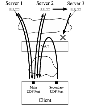
Figure 8: NAT Check Test Method for UDP
When server 2 receives a UDP request from the client, besides replying directly to the client it also forwards the request to server 3, which in turn replies to the client from its own IP address. If the NAT's firewall properly filters “unsolicited” incoming traffic on a per-session basis, then the client never sees these replies from server 3, even though they are directed at the same public port as the replies from servers 1 and 2.
To test the NAT for hairpin translation support, the client simply opens a second UDP socket at a different local port and uses it to send messages to the public endpoint representing the client's first UDP socket, as reported by server 2. If these messages reach the client's first private endpoint, then the NAT supports hairpin translation.
The TCP test follows a similar pattern as for UDP. The client uses a single local TCP port to initiate outbound sessions to servers 1 and 2, and checks whether the public endpoints reported by servers 1 and 2 are the same, the first precondition for reliable TCP hole punching.
The NAT's response to unsolicited incoming connection attempts also impacts the speed and reliability of TCP hole punching, however, so NAT Check also tests this behavior. When server 2 receives the client's request, instead of immediately replying to the client, it forwards a request to server 3 and waits for server 3 to respond with a “go-ahead” signal. When server 3 receives this forwarded request, it attempts to initiate an inbound connection to the client's public TCP endpoint. Server 3 waits up to five seconds for this connection to succeed or fail, and if the connection attempt is still “in progress” after five seconds, server 3 responds to server 2 with the “go-ahead” signal and continues waiting for up to 20 seconds. Once the client finally receives server 2's reply (which server 2 delayed waiting for server 3's “go-ahead” signal), the client attempts an outbound connection to server 3, effectively causing a simultaneous TCP open with server 3.
What happens during this test depends on the NAT's behavior as follows. If the NAT properly just drops server 3's “unsolicited” incoming SYN packets, then nothing happens on the client's listen socket during the five second period before server 2 replies to the client. When the client finally initiates its own connection to server 3, opening a hole through the NAT, the attempt succeeds immediately. If on the other hand the NAT does not drop server 3's unsolicited incoming SYNs but allows them through (which is fine for hole punching but not ideal for security), then the client receives an incoming TCP connection on its listen socket before receiving server 2's reply. Finally, if the NAT actively rejects server 3's unsolicited incoming SYNs by sending back TCP RST packets, then server 3 gives up and the client's subsequent attempt to connect to server 3 fails.
To test hairpin translation for TCP, the client simply uses a secondary local TCP port to attempt a connection to the public endpoint corresponding to its primary TCP port, in the same way as for UDP.
The NAT Check data we gathered consists of 380 reported data points covering a variety of NAT router hardware from 68 vendors, as well as the NAT functionality built into different versions of eight popular operating systems. Only 335 of the total data points include results for UDP hairpin translation, and only 286 data points include results for TCP, because we implemented these features in later versions of NAT Check after we had already started gathering results. The data is summarized by NAT vendor in Table 1; the table only individually lists vendors for which at least five data points were available. The variations in the test results for a given vendor can be accounted for by a variety of factors, such as different NAT devices or product lines sold by the same vendor, different software or firmware versions of the same NAT implementation, different configurations, and probably occasional NAT Check testing or reporting errors.
Table 1: User Reports of NAT Support for UDP and TCP Hole Punching
|              |                   UDP               |                TCP                |
|--------------|-------------------------------------|-----------------------------------|
|              | Hole               |                | Hole            |                 |
|--------------|--------------------|----------------|-----------------|-----------------|
|              | Punching | Hairpin |        |       | Punching        |  Hairpin        |
|--------------|----------|---------|--------|-------|---------|-------|--------|--------|
| NAT Hardware |          |         |        |       |         |       |        |        |
|--------------|----------|---------|--------|-------|---------|-------|--------|--------|
| Linksys      | 45/46    | (98%)   | 5/42   | (12%) | 33/38   | (87%) | 3/38   | (8%)   |
| Netgear      | 31/37    | (84%)   | 3/35   | (9%)  | 19/30   | (63%) | 0/30   | (0%)   |
| D-Link       | 16/21    | (76%)   | 11/21  | (52%) | 9/19    | (47%) | 2/19   | (11%)  |
| Draytek      | 2/17     | (12%)   | 3/12   | (25%) | 2/7     | (29%) | 0/7    | (0%)   |
| Belkin       | 14/14    | (100%)  | 1/14   | (7%)  | 11/11   | (100%)| 0/11   | (0%)   |
| Cisco        | 12/12    | (100%)  | 3/9    | (33%) | 6/7     | (86%) | 2/7    | (29%)  |
| SMC          | 12/12    | (100%)  | 3/10   | (30%) | 8/9     | (89%) | 2/9    | (22%)  |
| ZyXEL        | 7/9      | (78%)   | 1/8    | (13%) | 0/7     | (0%)  | 0/7    | (0%)   |
| 3Com         | 7/7      | (100%)  | 1/7    | (14%) | 5/6     | (83%) | 0/6    | (0%)   |
|--------------|----------|---------|--------|-------|---------|-------|--------|--------|
| OS-based NAT |          |         |        |       |         |       |        |        |
|--------------|----------|---------|--------|-------|---------|-------|--------|--------|
| Windows      | 31/33    | (94%)   | 11/32  | (34%) | 16/31   | (52%) | 28/31  | (90%)  |
| Linux        | 26/32    | (81%)   | 3/25   | (12%) | 16/24   | (67%) | 2/24   | (8%)   |
| FreeBSD      | 7/9      | (78%)   | 3/6    | (50%) | 2/3     | (67%) | 1/1    | (100%) |
|--------------|----------|---------|--------|-------|---------|-------|--------|--------|
| All Vendors  | 310/380  | (82%)   | 80/335 | (24%) | 184/286 | (64%) | 37/286 | (13%)  |
Out of the 380 reported data points for UDP, in 310 cases (82%) the NAT consistently translated the client's private endpoint, indicating basic compatibility with UDP hole punching. Support for hairpin translation is much less common, however: of the 335 data points that include UDP hairpin translation results, only 80 (24%) show hairpin translation support.
Out of the 286 data points for TCP, 184 (64%) show compatibility with TCP hole punching: the NAT consistently translates the client's private TCP endpoint, and does not send back RST packets in response to unsolicited incoming connection attempts. Hairpin translation support is again much less common: only 37 (13%) of the reports showed hairpin support for TCP.
Since these reports were generated by a “self-selecting” community of volunteers, they do not constitute a random sample and thus do not necessarily represent the true distribution of the NATs in common use. The results are nevertheless encouraging: it appears that the majority of commonly-deployed NATs already support UDP and TCP hole punching at least in single-level NAT scenarios.
There are a few limitations in NAT Check's current testing protocol that may cause misleading results in some cases. First, we only learned recently that a few NAT implementations blindly translate IP addresses they find in unknown application payloads, and the NAT Check protocol currently does not protect itself from this behavior by obfuscating the IP addresses it transmits.
Second, NAT Check's current hairpin translation checking may yield unnecessarily pessimistic results because it does not use the full, two-way hole punching procedure for this test. NAT Check currently assumes that a NAT supporting hairpin translation does not filter “incoming” hairpin connections arriving from the private network in the way it would filter incoming connections arriving at the public side of the NAT, because such filtering is unnecessary for security. We later realized, however, that a NAT might simplistically treat any traffic directed at the NAT's public ports as “untrusted” regardless of its origin. We do not yet know which behavior is more common.
Finally, NAT implementations exist that consistently translate the client's private endpoint as long as only one client behind the NAT is using a particular private port number, but switch to symmetric NAT or even worse behaviors if two or more clients with different IP addresses on the private network try to communicate through the NAT from the same private port number. NAT Check could only detect this behavior by requiring the user to run it on two or more client hosts behind the NAT at the same time. Doing so would make NAT Check much more difficult to use, however, and impossible for users who only have one usable machine behind the NAT. Nevertheless, we plan to implement this testing functionality as an option in a future version of NAT Check.
Despite testing difficulties such as those above, our results are generally corroborated by those of a large ISP, who recently found that of the top three consumer NAT router vendors, representing 86% of the NATs observed on their network, all three vendors currently produce NATs compatible with UDP hole punching [25]. Additional independent results recently obtained using the UDP-oriented STUN protocol [12], and STUNT, a TCP-enabled extension [8,9], also appear consistent with our results. These latter studies provide more information on each NAT by testing a wider variety of behaviors individually, instead of just testing for basic hole punching compatibility as NAT Check does. Since these more extensive tests require multiple cooperating clients behind the NAT and thus are more difficult to run, however, these results are so far available on a more limited variety of NATs.
UDP hole punching was first explored and publicly documented by Dan Kegel [13], and is by now well-known in peer-to-peer application communities. Important aspects of UDP hole punching have also been indirectly documented in the specifications of several experimental protocols, such as STUN [19], ICE [17], and Teredo [11]. We know of no existing published work that thoroughly analyzes hole punching, however, or that points out the hairpin translation issue for multi-level NAT (Section [3.5]).
We also know of no prior work that develops TCP hole punching in the symmetric fashion described here. Even the existence of the crucial SO_REUSEADDR/SO_REUSEPORT options in the Berkeley sockets API appears to be little-known among P2P application developers. NatTrav [4] implements a similar but asymmetric TCP hole punching procedure outlined earlier in Section [4.5]seq). NUTSS [9] and NATBLASTER [1] implement more complex TCP hole punching tricks that can work around some of the bad NAT behaviors mentioned in Section [5], but they require the rendezvous server to spoof source IP addresses, and they also require the client applications to have access to “raw” sockets, usually available only at root or administrator privilege levels.
Protocols such as SOCKS [14], UPnP [26], and MIDCOM [22] allow applications to traverse a NAT through explicit cooperation with the NAT. These protocols are not widely or consistently supported by NAT vendors or applications, however, and do not appear to address the increasingly important multi-level NAT scenarios. Explicit control of a NAT further requires the application to locate the NAT and perhaps authenticate itself, which typically involves explicit user configuration. When hole punching works, in contrast, it works with no user intervention.
Recent proposals such as HIP [15] and FARA [2] extend the Internet's basic architecture by decoupling a host's identity from its location [20]. IPNL [7], UIP [5,6], and DOA [27] propose schemes for routing across NATs in such an architecture. While such extensions are probably needed in the long term, hole punching enables applications to work over the existing network infrastructure immediately with no protocol stack upgrades, and leaves the notion of “host identity” for applications to define.
Hole punching is a general-purpose technique for establishing peer-to-peer connections in the presence of NAT. As long as the NATs involved meet certain behavioral requirements, hole punching works consistently and robustly for both TCP and UDP communication, and can be implemented by ordinary applications with no special privileges or specific network topology information. Hole punching fully preserves the transparency that is one of the most important hallmarks and attractions of NAT, and works even with multiple levels of NAT--though certain corner case situations require hairpin translation, a NAT feature not yet widely implemented.
The authors wish to thank Dave Andersen for his crucial support in gathering the results presented in Section [6]. We also wish to thank Henrik Nordstrom, Christian Huitema, Justin Uberti, Mema Roussopoulos, and the anonymous USENIX reviewers for valuable feedback on early drafts of this paper. Finally, we wish to thank the many volunteers who took the time to run NAT Check on their systems and submit the results.
-
Andrew Biggadike, Daniel Ferullo, Geoffrey Wilson, and Adrian Perrig.
NATBLASTER: Establishing TCP connections between hosts behind NATs.
In ACM SIGCOMM Asia Workshop, Beijing, China, April 2005. -
David Clark, Robert Braden, Aaron Falk, and Venkata Pingali.
FARA: Reorganizing the addressing architecture.
In ACM SIGCOMM FDNA Workshop, August 2003. -
S. Deering and R. Hinden.
Internet protocol, version 6 (IPv6) specification, December 1998.
RFC 2460. -
Jeffrey L. Eppinger.
TCP connections for P2P apps: A software approach to solving the NAT problem.
Technical Report CMU-ISRI-05-104, Carnegie Mellon University, January 2005. -
Bryan Ford.
Scalable Internet routing on topology-independent node identities.
Technical Report MIT-LCS-TR-926, MIT Laboratory for Computer Science, October 2003. -
Bryan Ford.
Unmanaged internet protocol: Taming the edge network management crisis.
In Second Workshop on Hot Topics in Networks, Cambridge, MA, November 2003. -
Paul Francis and Ramakrishna Gummadi.
IPNL: A NAT-extended Internet architecture.
In ACM SIGCOMM, August 2002. -
Saikat Guha and Paul Francis.
Simple traversal of UDP through NATs and TCP too (STUNT).
http://nutss.gforge.cis.cornell.edu/. -
Saikat Guha, Yutaka Takeday, and Paul Francis.
NUTSS: A SIP-based approach to UDP and TCP network connectivity.
In SIGCOMM 2004 Workshops, August 2004. -
M. Holdrege and P. Srisuresh.
Protocol complications with the IP network address translator, January 2001.
RFC 3027. -
C. Huitema.
Teredo: Tunneling IPv6 over UDP through NATs, March 2004.
Internet-Draft (Work in Progress). -
C. Jennings.
NAT classification results using STUN, October 2004.
Internet-Draft (Work in Progress). -
Dan Kegel.
NAT and peer-to-peer networking, July 1999.
http://www.alumni.caltech.edu/~dank/peer-nat.html. -
R. Moskowitz and P. Nikander.
Host identity protocol architecture, April 2003.
Internet-Draft (Work in Progress). -
NAT check.
http://midcom-p2p.sourceforge.net/. -
J. Rosenberg.
Interactive connectivity establishment (ICE), October 2003.
Internet-Draft (Work in Progress). -
J. Rosenberg, C. Huitema, and R. Mahy.
Traversal using relay NAT (TURN), October 2003.
Internet-Draft (Work in Progress). -
J. Rosenberg, J. Weinberger, C. Huitema, and R. Mahy.
STUN - simple traversal of user datagram protocol (UDP) through network address translators (NATs), March 2003.
RFC 3489. -
J. Saltzer.
On the naming and binding of network destinations.
In P. Ravasio et al., editor, Local Computer Networks, pages 311-317. North-Holland, Amsterdam, 1982.
RFC 1498. -
P. Srisuresh and M. Holdrege.
IP network address translator (NAT) terminology and considerations, August 1999.
RFC 2663. -
P. Srisuresh, J. Kuthan, J. Rosenberg, A. Molitor, and A. Rayhan.
Middlebox communication architecture and framework, August 2002.
RFC 3303. -
G. Tsirtsis and P. Srisuresh.
Network address translation - protocol translation (NAT-PT), February 2000.
RFC 2766. -
Justin Uberti.
E-mail on IETF MIDCOM mailing list, February 2004.
Message-ID: 402CEB11.1060906@aol.com. -
UPnP Forum.
Internet gateway device (IGD) standardized device control protocol, November 2001.
http://www.upnp.org/. -
Michael Walfish, Jeremy Stribling, Maxwell Krohn, Hari Balakrishnan, Robert Morris, and Scott Shenker.
Middleboxes no longer considered harmful.
In USENIX Symposium on Operating Systems Design and Implementation, San Francisco, CA, December 2004.
while read -r it ; do
    url=$(echo $it | sed -n "s/.\+(\(.\+\))\(.\+\)\?/\1/p")
    curl -s $url | /c/opendocs/html2md.ts | sed -n '/Navigation Menu/,/Related Posts/p' >> /c/opendocs/P2P_NAT_Traversal.md
done <<EOF
# [NAT](https://www.practicalnetworking.net/series/nat/nat/)
#   [Why NAT?](https://www.practicalnetworking.net/series/nat/why-nat/)
#   [NAT Terminology](https://www.practicalnetworking.net/series/nat/nat-terminology/)
#   [Static NAT](https://www.practicalnetworking.net/series/nat/static-nat/)
#   [Static PAT](https://www.practicalnetworking.net/series/nat/static-pat/)
#   [Dynamic PAT](https://www.practicalnetworking.net/series/nat/dynamic-pat/)
#   [Dynamic NAT](https://www.practicalnetworking.net/series/nat/dynamic-nat/)
#   [Policy NAT and Twice NAT](https://www.practicalnetworking.net/series/nat/policy-nat-twice-nat/)
#   [NAT Terminology Disambiguation](https://www.practicalnetworking.net/series/nat/nat-terminology-disambiguation/)
EOF
exit
Every device on the Internet has an IP address. The IP address serves as the device’s identification – much like how a phone number identifies a particular phone.
When devices communicate on the Internet, they are sending data from their IP address to the IP address of their intended destination.
Sometimes, while data is en route to a destination, the IP addresses used in the communication need to be translated to different IP addresses.
This IP translation is similar to when multiple employees of the same company use their individual phones (with individual phone numbers) to make outbound phone calls, yet still appear as if they were all using the same company phone number.
The process of translating one IP address to another is known as Network Address Translation, or NAT.
There are many different reasons one would need NAT, and many different ways of translating IP addresses. Understanding NAT is paramount to any Network Engineer, as every wifi, home, or company network employs Network Address Translation at some point.
This article series will clearly illustrate every type of address translation that exists in a thorough, but concise, manner that is entirely vendor agnostic and applies to the entire spectrum of address translation on the Internet.
Contents
- Why NAT?
- NAT Terminology
- Static NAT
- Static PAT
- Dynamic PAT
- Dynamic NAT
- Policy NAT and Twice NAT
- NAT Terminology Disambiguation
Before we can discuss how NAT works, we must discuss the purpose of NAT and answer the question, “Why NAT?”
In the original plan for the Internet, every host was meant to have its own unique IP address. This means if you had a network which had 30 hosts, you would need 30 unique IP addresses for each host to access the Internet, or to be accessed from the Internet.
IP addresses are a finite resource – 32 bits allows for roughly 4.2 billion possible IP address combinations.
As the Internet grew in popularity, the industry realized there would one day be more hosts on the Internet than there were IP addresses available.
The long term, permanent solution was to create a larger address range, and IPv6 was born which is an addressing scheme that uses 128 bits. However, transitioning to IPv6 would prove to be a complicated and slow process, so a short term solution had to also be implemented: RFC 1918 was created to reduce the rate of IPv4 address utilization and delay the inevitable exhaustion of addresses.
RFC 1918 designated three different address sets that were considered free to use and reuse by any organization:
10.0.0.0 /8– any IP address in the range of10.#.#.#172.16.0.0 /12– any IP address in the range of172.[16-31].#.#192.168.0.0 /16– any IP address in the range of192.168.#.#
These addresses were labeled as Private addresses, and were deemed unroutable on the Internet. All the remaining addresses remained Public addresses, and able to be routed on the Internet.
With RFC 1918, if you had 30 hosts on your network, all 30 of them would use 30 unique Private IP addresses, but for Internet facing traffic, all 30 could share a single Public address. Allowing you to conserve 29 Public addresses.
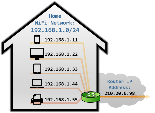
This is exactly what happens on WiFi networks. Whether it is a home WiFi network, or a coffee shop, or airport, each device on the network has a private IP address from one of the private ranges above. When these devices speak to the Internet, they all share the IP address assigned to the WiFi Router.
These Private addresses can be reused with each deployment without fear of duplicate addresses on the Internet. So long as the Public address(es) they are sharing are unique.

For example, a lot of home WiFi networks use the common range of 192.168.1.0/24 for each of their internal address ranges. The home Wifi router then translates each independent set of Private 192.168.1.0/24 addresses into unique Public addresses.
The idea is anyone can use these addresses, or even re-use these addresses, for as many hosts as they like on their internal network. NAT can then translate the multitude of hosts using Private addresses into a much smaller set of Public addresses – thereby curbing the rate of which IPv4 addresses are being utilized.
Private addresses are theoretically infinite, since they can be reused with each deployment. Public addresses are finite, and tracked by the Internet Authority for Assigned Numbers (IANA) to ensure no organization inadvertently uses duplicate Public addresses.
Consequently, the concept of Network Address Translation was born to facilitate the translation between Private addresses and Public addresses.
Traditionally, NAT exists to translate Private IPv4 addresses into Public IPv4 addresses. For the sake of simplicity, this article series will describe NAT from this perspective. However, in reality, it does not matter whether the IP addresses being translated are public or private. NAT could easily occur from private addresses to other private addresses or from public addresses to other public addresses.
As discussed before, Network Address Translation, or NAT, is a process that involves translating Private IP addresses into Public IP addresses. There are different operations within NAT and understanding each of them requires understanding NAT terminology.
Network Address Translation and Port Address Translation differ by modifying different headers in a data packet.

Network Address Translation, or NAT, implies a translation of an IP address to another IP address.
NAT in and of itself only affects the L3 header, which in today’s world will be the IPv4 header. While NAT can modify an IPv6 header as well, it really isn’t common, as IPv6 was created in such a way to avoid the need for NAT altogether.
Port Address Translation, or PAT, implies a translation of an IP address and Port to another IP address and Port.
PAT affects both the L3 header and the L4 header. Which means the IPv4 Header, as well as either the TCP or UDP header, will be modified.
You could consider PAT as a subset of NAT (i.e., Network Address Translation along with a Port translation), but there isn’t really a common use case for a Port translation only without an accompanying IP address translation as well. Therefore, nearly every instance of a PAT will also typically include an IP address translation as well.
In summary, a NAT modifies only the L3 header, and a PAT modifies both the L3 and L4 header. Or, said another way, a NAT modifies only the IP, and a PAT modifies both the IP and Port.
Both a NAT and a PAT can exist in two forms: Static or Dynamic. These two terms designate whether the post-translation attributes of the packet are explicitly defined by the administrator or determined by the translation device.
In either case, the pre-translation attributes are explicitly defined. This is how the NAT device knows which packets should be translated in the first place.
To help define the terms, we will look at an example of a Static translation and Dynamic translation below. The examples will use a Router as a NAT device, but many other devices can also perform address translation (Firewalls, Load Balancers, etc).
In a Static translation, the post-translation attributes are explicitly defined by the administrator (IP address for a NAT, or IP:Port for a PAT). A Static translation implies the pre-translation IP or IP:Port will permanently map to the same, constant post-translation IP or IP:Port.
In this example, only the IP address is changing (NAT), and the mapping between pre-translation and post-translation is permanent (Static) – the IP address 10.1.1.11 will always be translated to 73.8.2.11 (and vice versa). Hence, this is an example of a Static NAT.
A Static mapping is sometimes referred to as a One-to-One translation – implying that in a Static translation, a single IP or IP:Port can only ever appear as another single IP or IP:Port.
In a Dynamic translation, the post-translation attributes are selected by the router at the time that the packet is received – the final post-translation attributes are not permanently mapped to pre-translation attributes.
Of course, the scope of post-translation attributes must be defined by the administrator, but the exact mapping is determined by the device, at the time the packet is received.
In this example, both the IP address and the Port are changing (which makes this a PAT), and the mapping between the pre-translation and post-translation is not explicitly defined by the administrator (which makes this a Dynamic translation). Hence, this is an example of a Dynamic PAT.
When the packet from 10.1.1.11 arrived on the Router, the Router chose a new source port of 6667. When the packet from 10.1.1.22 arrived on the Router, the Router chose a new source port of 6668. Both hosts are sharing the public IP address 73.8.2.66.
There is no guarantee that the next connections initiated by either host will have port numbers of 6667 or 6668 – they will very likely be something else randomly chosen by the Router, at the time the next packet is received by the Router.
A Dynamic mapping is sometimes referred to as a One-to-Many or Many-to-One translation – implying that in a Dynamic translation, many addresses can appear as one, or one address can appear as many.
Both Static NAT and the Dynamic PAT will be explored in more detail in later articles in this series.
In total, we discussed two sets of two terms: NAT and PAT, and Static and Dynamic. When these are combined, they create four possible variants of Network Address Translation:
Each of the four combinations above account for every type of Network Address Translation that exists. They will also each be the subject of their own article in this series.
The typical use case for a Static NAT is for a Server on a Private IPv4 network to be reached externally from the Internet.
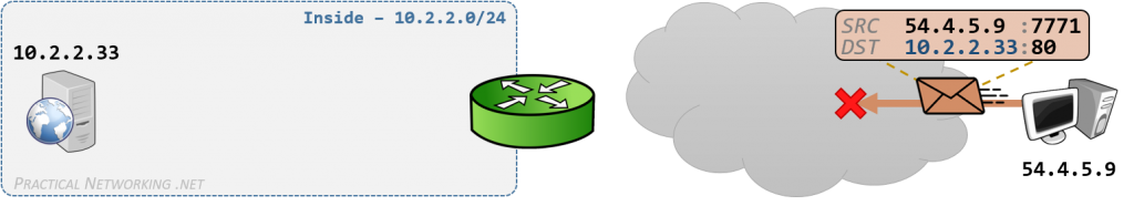
In this example, the Internet host **54.4.5.9** needs to connect to the web server on the Inside network. The web server is on an internal network and is therefore configured with the Private IP address of **10.2.2.33**.
If the Internet host attempts to send a packet to the IP address of the server (10.2.2.33), the packet will be dropped when it reaches the Internet. Recall, Private IP addresses are not routable on the Internet.
For a host on the Internet to reach the server, a Static NAT must be configured on the NAT device. In our example, the Router in front of the 10.2.2.0/24 network will be the NAT device, and we will configure it to translate the private IP address **10.2.2.33** to the Public IP address **73.8.2.33**.
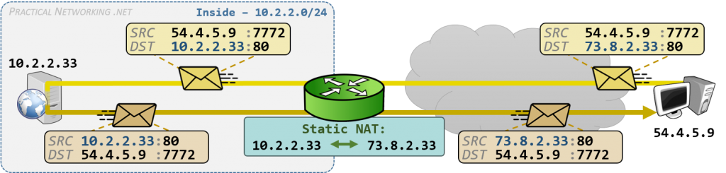
Now, the Internet host can send a packet to the correlating Public IP address (73.8.2.33) which will be routed through the Internet to the NAT device. The Router (acting as our NAT device) will then translate the packet to the Server’s private IP address (10.2.2.33). When the web server responds, the router will un-translate the packet back to the original IP address of 73.8.2.33.
The Static NAT allowed the internal host with the private IP address to be accessed by an external host.
With that in mind, there are three additional points that must be made regarding Static NAT.
Whether the Source or Destination of the packet is translated is dependent on the direction the packet is traveling. The inbound packet has its Destination IP translated (from the Internet to the server). The outbound packet has its Source IP translated (from the server to the Internet).
Either way, the one IP address 10.2.2.33 always maps to the one IP address 73.8.2.33. This is why a Static NAT is also sometimes called a [one-to-one] NAT.
If you had 30 servers on the Inside network, each with their own Private IP address, and you wanted to use Static NAT, then you would need 30 unique Public IP addresses for the translations.
We discussed earlier that the [original intent of Network Address Translation was to conserve Public IPv4 addresses]. However, as you can see, a Static NAT does not actually conserve any Public IPv4 addresses. Instead, the primary purpose of a Static NAT is to [expose a server with a Private IP address] to the public Internet.
Finally, in the example above, the initial packet was sent from the Internet host. But it could have easily been sent from the server on the Inside network. Regardless of who initiated the connection, the Static NAT would cause the Source of the outbound packets or the Destination of the inbound packets to be translated.
The key point is that a Static NAT translation is bidirectional. Whether the internal host or the external host sent the first packet, it would “pass through” the Static NAT. There are variations of NAT which we will discuss later in this article series where the translation will not be bidirectional.
According to the definitions outlined in the [NAT Terminology] article, a Static PAT implies a translation of the [IP address and Port], where the [post-translation attributes are explicitly defined].
There are multiple use cases for a Static PAT, but they all have one thing in common – a need to manually change the TCP or UDP port as a packet moves through a router or firewall.
One specific use case for Static PAT is to use a single Public IP address to host multiple services on different internal servers. This is in contrast with a [Static NAT] which would only allow you to use a single Public IP address to host multiple services on the same server.
This illustration will show how Static PAT can enable the single IP address 73.8.2.44 to host two different services (HTTP and HTTPS) using two separate internal servers (10.4.4.41 and **10.4.4.42**):
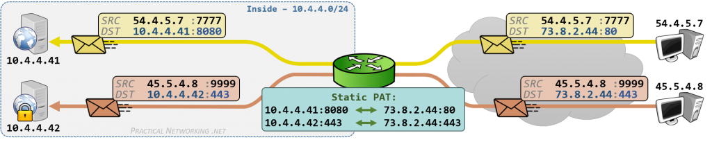
The Router is acting as our translation device and is configured with two Static PAT entries. Since these are [static] translations, the mapping is explicitly defined: 73.8.2.44:80 will always be translated to **10.4.4.41:8080** and 73.8.2.44:443 will always be translated to **10.4.4.42:443**.
Two hosts somewhere on the Internet both make a request to the same IP address (73.8.2.44) – one request using **HTTP** (port 80), one request using **HTTPS** (port 443). When their packets arrive on the Router, they get translated and sent to two different servers for processing.
The single Public IP address (**73.8.2.44**) is hosting two services (HTTP and HTTPS) served by two different internal servers (10.4.4.41 and **10.4.4.42**).
If you use a Static PAT in this way (where one public IPv4 address is used to host multiple services on multiple servers), then you are conserving IPv4 address space. You could theoretically have 10 (or 50, or 200, or 1000+) different servers, each hosting a different service, all using a single Public IPv4 address.
The same illustration above also provides yet another use case for Static PAT – the **10.4.4.41** server is hosting HTTP traffic on a non-standard port (**8080**).
Without the port translation, hosts on the Internet would have to specify the non-standard port in their web browser by visiting “www.site.com:8080”. Instead, with the Static PAT, the users can just type “www.site.com” (which implicitly assumes the standard web port of **80**) and the router automatically translates the packet to port **8080** instead.
This could work in reverse as well. Where a non-standard port is used on the outside, but a standard port is used on the inside server.
For example, the standard port associated with SSH traffic is TCP/22. Malicious users routinely scan the entire IPv4 address space for servers listening on port TCP/22 to look for all SSH servers in hopes of finding some with weak passwords. A common strategy is to host SSH on a non-standard port in an effort to hide your SSH server from this mass scanning that occurs on port 22.
The response traffic from these hosts would be untranslated by the router. Since this is the outbound traffic, the source of the packet will be translated. Whereas on the inbound packet above, the destination of the packet was translated.

Once again, since the pre-translation IP:Port and post-translation IP:Port in a Static PAT are explicitly defined, the initial packet could have come from either the Internet hosts or the inside hosts. Therefore, a Static PAT translation is [bidirectional].
There is one final use-case for Static PAT, which is possibly the least common of the three. A Static PAT allows you to selectively “punch holes” through a particular Public IP address.
When we looked at a [Static NAT], only the IP address is translated – the port numbers are left untouched. Which means, every port is explicitly mapped to every port. It’s possible that you may want only ports 80 and 443 to get through, but not port 21 or 23 (or any other). A Static NAT does not allow you to choose.
Whereas instead, with a Static PAT, if you only create a translation for port 80 and 443, only those paths through the router will exist. Protecting your internal servers from unwanted access attempts.
In this context, Static PAT is sometimes referred to as Port Forwarding: a specific port on an external address is forwarded to a specific port on an internal address.
Admittedly, the same effect can be attained by creating a Static NAT and applying an access-list or security policy to only allow the desired traffic through. As such, this is a use-case for Static PAT, but by no means is it the only way to attain the same effect.
The most common usage of selectively punching holes is to create a _bi_directional path through _uni_directional NAT translation. This will make more sense when we discuss Dynamic PAT in the next article.
According to the definitions outlined in the [NAT Terminology] article, a Dynamic PAT implies a translation of the [IP address and Port], where the [post-translation attributes are selected by the router].
Dynamic PAT is the most common of the [types of address translation] we will discuss in this article series. Dynamic PAT is used any time multiple internal hosts need to share a single public IP address.
On a small scale, this is exactly what your home Wi-Fi router does. You may have [5-25 unique devices on your home network], each of them with their own private IP address. But when any of them try to speak with the Internet, [they all share the single, unique public IP address assigned to your router]).
The same type of translation happens with the Wi-Fi at coffee shops, or restaurants, or airports. This was the exact same example that was provided in the “[Why NAT]?” article – the illustrations are examples of a Dynamic PAT.
Of all the types of Network Address Translation, a Dynamic PAT is the most conducive to conserving IP address space. It is not uncommon to have hundreds of internal hosts sharing one public IP address.
Dynamic PAT is often referred to as a [many-to-one or one-to-many] translation, implying the many hosts on the Wi-Fi network are sharing the one Public IP address on the Internet.
Of course, this simple example referred to earlier hasn’t quite shown how ports are translated, or how the Router selected the post-translation attributes. To illustrate those concepts, we will have to look at the packet flow through a Dynamic PAT in more detail.
The image below illustrates what is occurring at the packet level:
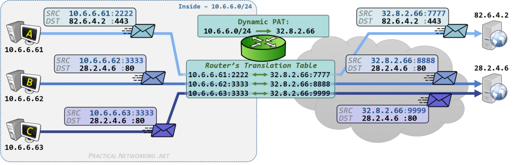
The Router is serving as our translation device, and is configured with a Dynamic PAT which translates any IP address on the Inside network (**10.6.6.0/24**) to the IP address **32.8.2.66**. When packets are translated, the Router makes note of the attributes of the original and translated packet in the Router’s Translation Table.
Hosts A, B, and C each send a packet. They each use their own, unique Private IP address as the Source IP address, and they each randomly select a Source Port.
There are approximately 60,000 port numbers that can be chosen, and it is entirely feasible for two different hosts to randomly select the same source port (as is the case with Host B and Host C above).
Notice the configuration of the Dynamic PAT does not include specifying a port number. Even though the ports are not explicitly set in the Router’s configuration, this translation is still classified as a PAT because the port is dynamically changed by the Router.
In our example above, upon reception of each packet, the Router translates the source IP address of each packet to **32.8.2.66** (as explicitly configured), and randomly selects a new, unique source port number for each packet (**7777**, **8888**, and **9999**). The Router translated the port (PAT) and the Router selected the new source port (Dynamic).
Each specific mapping is recorded in the Router’s Translation Table. This translation table will be used to “un-translate” the response packets when they return from the Internet.
When the two webservers respond to the three packets illustrated in the example above, the packet flow will resemble the following:
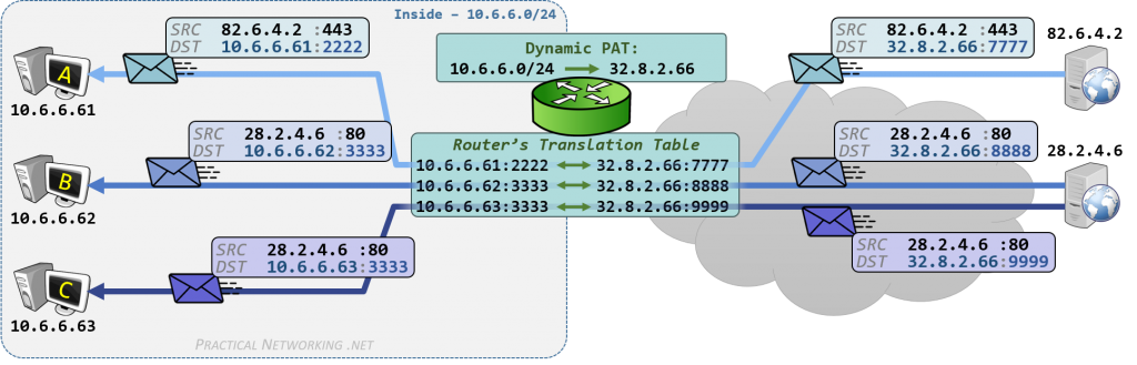
The response traffic from the web servers simply reverses the source and destination from the [initial packet]. Each web server sends the response traffic to the destination of the shared IP address (32.8.2.66), with the destination port number which the Router had selected in the original outbound traffic.
When the packets arrive on the Router, it matches them against the translation table to know how to “un-translate” the packet to their original attributes to get them to the appropriate host:
- The response packet sent to
32.8.2.66:**7777**is forwarded to Host A (10.6.6**.61:2222**) - The response packet sent to
32.8.2.66:**8888**is forwarded to Host B (10.6.6**.62:3333**) - The response packet sent to
32.8.2.66:**9999**is forwarded to Host C (10.6.6**.63:3333**)
In the last section, we pointed out that the router selected a new, random source port for the outbound packet. This re-randomizing of the source port is crucial to enabling successful communication through a Dynamic PAT.
Had the router not re-randomized the source port number, the outbound post-translation packets from Host B and Host C would have looked identical – they both would have had a Source IP of **32.8.2.66** and a Source port of **3333**.
Which means the response traffic for both packets from the **28.2.4.6** server would have looked identical – the Destination IP would have been 32.8.2.66 and the Destination port would have been **3333**.
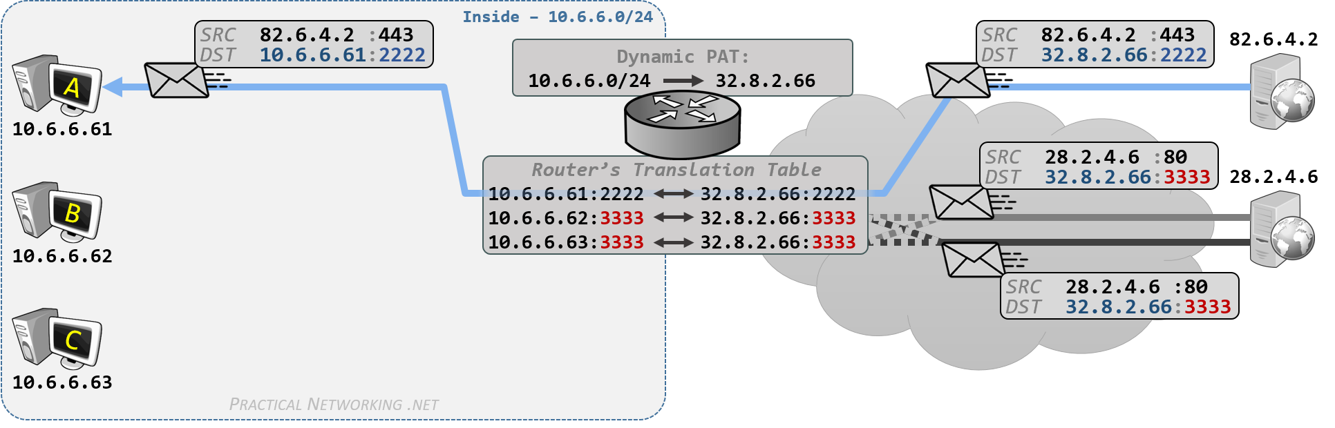
When the identical packets arrive, the router would have no way of distinguishing which packet should be untranslated to Host B (10.6.6.62) or which should be translated to Host C (10.6.6.63). The router would have no choice but to drop both packets.
This would cause packets to drop anytime two hosts happen to pick the same source port, which happens often enough that no host would be content with the connectivity (or lack thereof) provided through a Dynamic PAT.
For this reason, it is imperative that the Router ensures every packet sent through a Dynamic PAT uses a unique source port number. This allows the return packets to be distinguishable from one another, and allows the Router to forward the return traffic to the appropriate host.
Some NAT devices assure unique source ports by re-randomizing the source port for all connections when doing a Dynamic PAT translation. Some NAT devices do this by re-randomizing the source port only when duplicate ports are chosen by the inside hosts.
Regardless of the method used, so long as each connection’s packets can be identified by both unique IP Address and Port, for both Source and Destination, the response traffic can be successfully un-translated to the appropriate initial host.
As discussed before, a Dynamic PAT allows many internal hosts to share the same the same public IP address. One of the side effects of multiple hosts sharing a single IP address is the translation only works in one direction.
In the example above, Hosts A, B, and C initiated some traffic to external hosts. When the external hosts responded, the Router had entries in its translation table which allowed it to “un-translate” the packets and send them to the appropriate hosts.
If, however, a new connection was initiated from an external host and destined to the shared IP address, the router will have no way of knowing which internal host was the intended target of the packet.
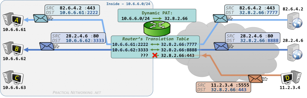
Not knowing whom to deliver the packet to, the Router has no choice but to drop the packet. As such, a Dynamic PAT only succeeds if the internal host sends the first packet. If the external host sends the first packet, it will be dropped when it reaches the translation device.
This is what is meant by a Dynamic PAT being a unidirectional translation – traffic will flow through a Dynamic PAT only if the internal host initiates the connection.
This is in contrast to [Static NAT] and [Static PAT], which are both bi-directional – traffic can be translated whether it was initiated by the external host or the internal host.
Keep in mind, this is not a “feature” of Dynamic PAT so much as it is a “side effect” of multiple hosts sharing a single IP address. Since it is possible for hosts to pick [identical source ports], the [router must change the source port during the translation], which means the [packets arriving from the Internet can only make it back through the Dynamic PAT due to the entry in the translation table], which [a packet initiated from an external network would not have].
If there is a need for certain ports to be accessible through a shared IP address, this can be achieved by using a Static PAT to [selectively punch holes] through the shared address of a Dynamic PAT.
According to the definitions outlined in the [NAT Terminology] article, a Dynamic NAT implies a translation of just the [IP address], where the [post-translation attributes are selected by the router].
In a Dynamic NAT, a multitude of hosts with private IP addresses can share an equal or fewer amount of public IP addresses.
It may seem very similar to a Dynamic PAT, but the major difference is this is a NAT – the port number is not changing, only the IP address. Which means a single public IP address cannot be shared among multiple internal Hosts at the same time ([as occurs with a Dynamic PAT]).
It is best explained with an illustration.

In the image we have a Router with an Inside network (10.7.7.0/24) with four hosts (.71, .72, .73, .74). The Router is configured with a Dynamic NAT which states the hosts on the Inside network can share three public IP addresses: 54.5.4.1, 54.5.4.2, and 54.5.4.3.
Host A (10.7.7.71) initiates a connection to 86.8.6.6, and the Router assigns Host A the public IP 54.5.4.1.
Host B (10.7.7.72) initiates a connection to 86.8.6.7, and the Router assigns Host B the public IP 54.5.4.2.
Host C (10.7.7.73) initiates a connection to 86.8.6.8, and the Router assigns Host C the public IP 54.5.4.3.
At this point, all the shared IP addresses have been used. Because of this, when Host D (10.7.7.74) attempts to initiate a connection to 86.8.6.9, the packet is dropped because there are no available public IP addresses the router can use to translate Host D’s private IP address.
While Host A/B/C have active connections through the Dynamic NAT, communication to those hosts are [Bidirectional]. Which means any host on the Internet can send packets to 54.5.4.1, .2, and .3 to reach Host A/B/C, respectively. We will expand on this in a moment.
When Host A is finished with its connection, the IP address it was assigned (54.5.4.1) becomes available again for the next internal host to use:

Here, we see Host D can now initiate a connection through the Dynamic NAT and receives the next available IP address.
In all cases, since this is a Dynamic NAT, only the IP address changed – the source port picked by the internal host remains the source port in the packet after translation.
Additionally, a Dynamic NAT has the potential to conserve IP addresses if configured as above where multiple internal hosts are sharing fewer Public IP addresses. However, you’ll see in a moment that Dynamic NAT is not always configured in that fashion.
The main use case for a Dynamic NAT is that while the translation is active it has the benefit of being [bidirectional], just like a [Static NAT].
For example, in the images above, Host B (**10.7.7.72**) has an active connection and was assigned the public IP address 54.5.4.2. So long as the connection is active in the Router’s translation able, any host on the Internet can send packets to 54.5.4.2 and they will reach Host B.
In a way, a Dynamic NAT assigns a temporary “dedicated IP” to each internal host (so long as IP addresses are available). Or, said another way, a Dynamic NAT creates a temporary [Static NAT].
There are two primary use cases for Dynamic NAT. The first is to allow for protocols which create a secondary, dynamic connection back to the client. The second is if you need a Bidirectional mapping of Private IPs to Public IPs, but don’t particularly care about the explicit mapping between the two.
The initial intent of a Dynamic NAT was to allow for protocols which create a second, dynamic connection back to the client. The main example of which is the File Transfer Protocol, or FTP.
FTP clients initiate outbound connections to FTP servers over destination port TCP/21. This connection serves as what FTP considers the control channel.
Over the control channel, a FTP client makes a request for a file and provides a random port number to the Server. The FTP Server then initiates a second connection back to the client from source port TCP/20, to the destination port provided by the client in the control channel. It is over this second connection that the file is actually transferred – this second connection is what FTP considers the data channel.
The issue is the data channel is a connection initiated from an external host on the Internet, destined to a host behind the Router. In a [Dynamic PAT], which [only allows connections initiated from the internal hosts], the data channel connection would be dropped.
But with a Dynamic NAT, the inbound data channel connection would be able to pass through the translation and the clients on the Inside server would be able to successfully use FTP to access files on the Internet.
The above describes the classic implementation of FTP known as Active FTP. There is a more modern implantation of FTP known as Passive FTP which does not require FTP clients to sit behind a Dynamic NAT, and instead allows them to sit behind the much more ubiquitous [Dynamic PAT].
Beyond the case of dynamic protocols described above, one other usage for a Dynamic NAT is if you have an equal number of Public IP addresses as you do Private hosts, and don’t particularly care which host get which public IP address, so long as each host gets one.
An example of such a case would be if the Router above could be configured to Dynamic NAT the entire 10.7.7.0/24 network into the entire 54.5.4.0/24 network. All 256 IP addresses in the Private range would receive an associated IP address on the Public range.
This would be the same effect of creating 256 individual [Static NAT] entries, except since the Dynamic NAT is Dynamic, there wouldn’t be an explicit mapping of a Private IP to a Public IP. The [Router would be choosing] which Private addresses map to which Public addresses.
If a particular deployment doesn’t necessarily care for a permanent, explicit mapping of private to public IP addresses, then Dynamic NAT could be used as a type of short cut to configuring 256 individual Static NAT entries.
When configured in this manner, a Dynamic NAT does not actually conserve any IP addresses, since it would be necessary to have a public IP address for each private host.
Despite the potential use cases outlined above, in the grand scheme of things, a Dynamic NAT is the least common [type of translation] deployed. This is due to the mapping created by a Dynamic NAT being temporary by nature, and therefore inconsistent.
In the [first illustration] above, Host A/B/C received the IP addresses **54.5.4.1**, **54.5.4.2**, **54.5.4.3** respectively. A moment later, in the second illustration, Host A’s connection terminated, and Host D received the IP address **54.5.4.1**. If a moment after that, Host A attempted to communicate, there would be no available IP addresses and Host A’s packet would be dropped:
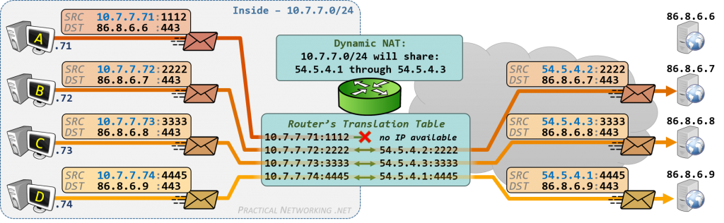
From Host A’s perspective, there was connectivity one moment, and no connectivity the next. This creates a generally poor experience for the user. And some of the most difficult for the network administrator to troubleshoot, as the connectivity issue is intermittent.
Of course, running out of available addresses and losing connectivity would only occur when there are less public IP addresses available in your translation pool than you have internal hosts – as is the case above with four internal hosts sharing three public IP addresses.
If you had a similar number of internal hosts and external IP addresses, as discussed in our [second use-case example], you wouldn’t run into the inconsistent connectivity problem. However, you would still run into the issue of inconsistent IP addresses.
For example, if there were no Host D in our illustration and there were just Hosts A/B/C sharing the IP addresses **54.5.4.1**, **54.5.4.2**, **54.5.4.3**. Host A may get **54.5.4.1** for the first connection, **54.5.4.2** for the next, and **54.5.4.3** for the third. At any given time, Host A would have connectivity, but there is no telling which public IP address Host A would receive at any given time.
Strictly speaking, this isn’t intrinsically a bad thing if you are using a Dynamic NAT for the specific case [described above] where you don’t necessarily need an explicit mapping.
But non-deterministic configurations can lead to unexpected and unintended results. So as a general rule in the Network Engineering field, deterministic designs are more favorable than non-deterministic designs.
Hence, if you have the public IP addresses available to give each of your private hosts a unique address, it is generally looked at as more favorable to configure multiple [Static NAT] translations instead of a single Dynamic NAT.
It should be noted that often when discussing address translation people will use the term Dynamic NAT when they actually mean Dynamic PAT. For the [reasons mentioned]above, Dynamic NAT is rarely used in production. If a single IP address is shared among many internal users, and if the port number changes, than it is indeed a [Dynamic PAT].
Every [type of NAT] we have discussed so far have two things in common. The first is that only the source of the packet is used to make a NAT decision. The second is that only the source of the outbound packet is translated. Policy NAT and Twice NAT are two ways of performing any type of NAT that expand beyond these two facts.
First, let’s quickly recap what we learned in the previous articles:
[NAT vs PAT] – these terms define whether just the IP address portion of the packet, or the IP address and Port number are being translated
[Static vs Dynamic] – these terms define whether the post-translation attributes are explicitly defined by the administrator, or ephemerally determined by the router.
When combined, this provides four possible variations of Network Address Translation:
- [Static NAT] – Translation of just the IP address where the administrator explicitly defines the IP address after translation
- [Static PAT] – Translation of the IP address and Port, where the administrator explicitly defines the IP address and Port after translation
- [Dynamic PAT] – Translation of the IP address and Port, where the router determines the new IP address and Port after translation
- [Dynamic NAT] – Translation of just the IP address, where the router determines the new IP address after translation
To configure each type of NAT above, we must define for the router exactly what traffic should be translated, and what it should be translated to.
If we review the configuration applied in the Static NAT or Dynamic PAT articles, we essentially instructed the Router to perform the following translations:
- If the source IP address is
10.2.2.33, translate the source IP statically to73.8.2.33 - If the source IP address is
10.6.6.0/24translate the source IP to32.8.2.66and dynamically pick a unique Source port
Notice in both cases we are making a decision to perform address translation based solely upon matching the source IP address of the packet – the destination address was not considered.
This is fine if you want all traffic from the Inside servers translated the same way for every destination they may speak to. However, there are times when you want to translate traffic to a certain destination one way, then translate traffic to a different destination a completely different way.
In such cases, when you need to conditionally translate traffic based upon the destination of the packet, you will need to use what is known as a Policy NAT.
The following example is the [same illustration as we used in the Dynamic PAT], except we’ve added one additional, conditional translation to the configuration:

There are two parts to the Router’s configuration. The first part of the configuration produces this behavior:
- If the source IP address is
**10.6.6.0/24**and the destination IP address is**45.5.4.9**, translate the source IP using Dynamic PAT to the address**32.8.2.77**
The additional configuration tells the router to translate a packet based upon the criteria of matching both the Source and Destination of the packet. In the industry, this is referred to as a Policy NAT.
A Policy NAT is simply any of the [four NAT types we discussed prior in this article series], except the [NAT decision] requires matching both the Source and Destination of a packet.
By contrast, every example of address translation thus far made a NAT decision based upon only the source of the packet.
The specific illustration immediately above was an example of a Policy Dynamic PAT – A translation decision based upon matching the source and destination of the packet ([Policy]), with the router determining the attributes after translation ([Dynamic]), which translated the source IP address and port ([PAT]).
The second part of the configuration produces this behavior:
- If the source IP address is
**10.6.6.0/24**, and the destination IP address is<**any**thing>, translate the source IP using Dynamic PAT to the address**32.8.2.66**
The second configuration item in the illustration above is simply a regular, [Dynamic PAT].
Every traditional Dynamic PAT implies matching for any destination. Whereas the Policy Dynamic PAT in the [first example] would only match for specific destinations.
In each example of the traditional [four types of NAT] we’ve discussed in this article series, only one “side” of the packet was being modified: the Source of the outbound packet or the Destination of the inbound packet.
Moreover, in the prior section we discussed Policy NAT: making a NAT decision based upon matching both the source and destination of traffic. However, even in a Policy NAT, once the decision was made, only one side of the packet was being modified.
If you refer back to the [Policy Dynamic PAT example], when Host A (**10.6.6.61**) was speaking to the Server, we translated **10.6.6.61** using a Dynamic PAT into **32.8.2.77**. Notice the Server’s IP address (**45.5.4.9**) was never translated, only the client’s – only one side of the packet was changed (the source of the outbound packet).
There are occasions where you need to translate both sides of the packet – this type of translation is referred to as a Twice NAT. The term comes from the fact that you are performing NAT twice: once on the source of the packet and another time on the destination of the packet.
There are many use cases for Twice NAT, we will provide one examples below. Another example will be illustrated in a separate article.
At the core of it, a Twice NAT is a type of NAT where both the Source and Destination of the packet will be translated. Take this scenario as an example.
You are in charge of a Router with hosts on a private network (**10.6.6.0/24**) that have chosen to use Google’s Public DNS Resolving Server (**8.8.8.8**). However, company policy states DNS requests must be made using the Corporate DNS server (**32.9.1.8**). One option is to manually verify every user’s DNS configuration, but that does not scale. Instead, another option would be to translate any outbound requests to **8.8.8.8** into a request for **32.9.1.8**.
Notice the configuration is making a decision based upon matching a Source of **10.6.6.0/24** and a Destination of **8.8.8.8** – this makes the configuration a Policy NAT. Furthermore, the configuration is translating the source using a Dynamic PAT, and the destination using a Static NAT – this makes the configuration a Twice NAT, since we are doing two instances of address translation.
The packet sent by the host is sourced from a private IP address and destined to Google’s DNS servers. But after crossing the router, the packet is now sourced from a public IP address and destined to the Corporate DNS servers.
The internal host is still configured to use Google’s DNS servers, but their traffic is automatically being redirected to the corporate DNS servers. The internal host will not know that anything is different, and unless they go out of their way to validate the DNS responses, they will have no idea that the response is coming from the corporate DNS server and not Google’s DNS server.
In this article, we unpacked and compared the ideas of a Policy NAT and a Twice NAT. As a quick summary:
- A Policy NAT is [any translation] that occurs based upon matching both the Source and Destination of traffic.
- A Twice NAT is [any translation] that involves translating both the Source and Destination of traffic.
These two terms can be combined, giving us a Policy Twice NAT. Which is a type of NAT which makes a decision based upon the Source and Destination of a packet ([Policy NAT]), and translates both the Source and Destination of a packet ([Twice NAT]).
If you’ve made it here, then at this point you should have a solid understanding of each of the [four types of translation] that can exist: [Static NAT], [Static PAT], [Dynamic PAT], and [Dynamic NAT]. Moreover, you have an understanding of [Policy NAT] and [Twice NAT], which are simply two different ways of implementing the four types of NAT.
The definitions and examples provided in this article series encompass every type of address translation that can possibly exist. That said, for marketing efforts, most vendors use their own distinct terminology to refer to each type of NAT we have discussed.
The purpose of this article is to provide a single page which lists all the types of address translation and what each vendor calls them. In the future, each vendor term will also link to a configuration guide for that specific vendor’s syntax and implementation.
|-----------|----------------|---------------------|---------------|--------------|
| Static NAT | Static PAT | Dynamic PAT | Dynamic NAT | |
|---|---|---|---|---|
| RFC 2663 | Static Address | Realm Specific | NAPT | Basic NAT |
| Assignment | Address and Port IP | |||
| ----------- | ---------------- | --------------------- | --------------- | -------------- |
| Wikipedia | Full Cone NAT | Full Cone NAT | Symmetric NAT | Restricted |
| Cone NAT | ||||
| ----------- | ---------------- | --------------------- | --------------- | -------------- |
| Cisco | Static NAT | Static PAT | Dynamic PAT | Dynamic NAT |
| Routers | ||||
| ----------- | ---------------- | --------------------- | --------------- | -------------- |
| Cisco | Static NAT | Static PAT | Dynamic PAT | Dynamic NAT |
| ASA/ASA-X | ||||
| ----------- | ---------------- | --------------------- | --------------- | -------------- |
| F5 LTM | NAT | Virtual Server | SNAT | n/a |
| ----------- | ---------------- | --------------------- | --------------- | -------------- |
| Juniper | Static NAT | Static NAT | Source NAT | Source NAT |
| with Port Mapping | with Disable | |||
| PAT Argument | ||||
| ----------- | ---------------- | --------------------- | --------------- | -------------- |
RFC 2663
- Static Address Assignment
- Realm Specific Address and Port IP
- Network Address Port Translation (NAPT)
- Basic NAT
Wikipedia
https://www.practicalnetworking.net/series/packet-traveling/packet-traveling/
while read -r it ; do
    url=$(echo $it | sed -n "s/.\+(\(.\+\))\(.\+\)\?/\1/p")
    curl -s -L $url | /c/opendocs/html2md.ts | sed -n '/Navigation Menu/,/Related Posts/p' >> /c/opendocs/P2P_NAT_Traversal.md
done <<EOF
# [](https://www.practicalnetworking.net/series/packet-traveling/packet-traveling/)
#  [](https://www.practicalnetworking.net/series/packet-traveling/osi-model/)
#  [](https://www.practicalnetworking.net/series/packet-traveling/key-players/)
#  [](https://www.practicalnetworking.net/series/packet-traveling/host-to-host/)
#  [](https://www.practicalnetworking.net/series/packet-traveling/host-to-host-through-a-switch/)
#  [](https://www.practicalnetworking.net/series/packet-traveling/host-to-host-through-a-router/)
#  [](https://www.practicalnetworking.net/series/packet-traveling/host-switch-router-switch-host/)
#  [](https://www.practicalnetworking.net/series/packet-traveling/packet-traveling-series-finale/)
EOF
exit
If you’re reading this blog, then you are no doubt already familiar with the wondrous creation that is the Internet. The Internet allows computers from all over the world to speak to each other.
When data leaves your computer, it is grouped into small chunks called Packets. These packets are essentially little envelopes that carry data across the Internet.
This article series is going to explain everything that happens to get one of these Packets from one side of the Internet to the other. We will look at each device and every step involved with a packet traveling across the Internet.
First, we’ll take a look at some background information on each separate function of network communication. Then we’ll take a look at the individual devices that perform each function. We will then tie everything together as we look at everything that happens for communication to happen between two computers with various interconnected devices.
- OSI Model
- Key Players
- Host to Host communication
- Host to Host communication through a Switch
- Host to Host communication through a Router
- Host to Switch to Router to Switch to Host
After reading through this article series on Packet Traveling, you will be able to understand and explain all the different events which occur in sending data from one side of the Internet to the other.
The Open Systems Interconnect model (OSI Model) explains all the individual functions that are necessary for the Internet to work.
It is a set of seven independent functions which combine to accomplish the end-goal of Computer to Computer communication.
Much like a car is composed of independent functions which combine to accomplish the end-goal of moving the car forward: A battery powers the electronics, an alternator recharges the battery, an engine rotates a driveshaft, an axle transfers the driveshaft’s rotation to the wheels, and so on and so forth.
Each individual part can be independently replaced or worked on, and as long as each individual part is functioning properly, the car moves forward.
The OSI model is divided into seven different layers, each of which fulfills a very specific function. When combined together, each function contributes to enables full computer to computer data communication.
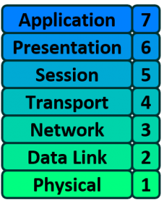
In the rest of this article, we will look at each of the individual layers of the OSI model and their individual responsibility.
The Physical layer of the OSI model is responsible for the transfer of bits — the 1’s and 0’s which make up all computer code.
This layer represents the physical medium which is carrying the traffic between two nodes. An example would be your [Ethernet cable] or Serial Cable. But don’t get too caught up on the word “Physical” — this layer was named in the 1970s, long before wireless communication in networking was a concept. As such, WiFi, despite it not having a physical, tangible presence, is also considered a Layer 1 protocol.
Simply put, Layer 1 is anything that carries 1’s and 0’s between two nodes.
The actual format of the data on the “wire” can vary with each medium. In the case of Ethernet, bits are transferred in the form of electric pulses. In the case of Wifi, bits are transferred in the form of radio waves. In the case of Fiber, bits are transferred in the form of pulses of light.
Aside from the physical cable, Repeaters and Hubs also operate at this layer.
A Repeater simply repeats a signal from one medium to the other, allowing a series of cables to be daisy chained together and increase the range a signal can travel beyond the single cable limit. These are commonly used in large WiFi deployments, where a single WiFi network is “repeated” throughout multiple access-points to cover a larger range.
A Hub is simply a multi-port Repeater. If four devices are connected to a single Hub, anything sent by one device gets repeated to the other three.
The Data Link layer of the OSI model is responsible for interfacing with the Physical layer. Effectively, Layer 2 is responsible for putting 1’s and 0’s on the wire, and pulling 1’s and 0’s from the wire.
The Network Interface Card (NIC) that you plug your Ethernet wire into handles the Layer 2 functionality. It receives signals from the wire, and transmits signals on to the wire.
Your WiFi NIC works the same way, receiving and transmitting radio waves which are then interpreted as a series of 1’s and 0’s.
Layer 2 will then group together those 1’s and 0’s into chunks known as Frames.
There is an addressing system that exists at Layer 2 known as the Media Access Control address, or MAC address. The MAC address uniquely identifies each individual NIC. Each NIC is pre-configured with a MAC address by the manufacturer; in fact, it is sometimes referred to as the Burned In Address (BIA).
Aside from your NIC, a Switch also operates at this layer. A Switch’s primary responsibility is to facilitate communication within Networks (this idea will be expanded upon in [a later article] in this series).
The overarching function of the Data Link layer is to deliver packets from one NIC to another. Or to put it another way, the role of Layer 2 is to deliver packets from hop to hop.
The Network layer of the OSI model is responsible for packet delivery from end to end.
It does this by using another addressing scheme that can logically identify every node connected to the Internet. This addressing scheme is known as the Internet Protocol address, or the IP Address.
It is considered logical because an IP address is not a permanent identification of a computer. Unlike the MAC address which is considered a physical address, the IP address is not burned into any computer hardware by the manufacturer.
Routers are Network Devices that operate at Layer 3 of the OSI model. A Router’s primary responsibility is to facilitate communication between Networks. As such, a Router creates a boundary between two networks. In order to communicate with any device not directly in your network, a router must be used.
The interaction and distinction between Layer 2 and Layer 3 is crucial to understanding how data flows between two computers. For example, if we already have a unique L2 addressing scheme on every NIC (like MAC addresses), why do we need yet another addressing scheme at L3 (like IP addresses)? Or vice versa?
The answer is that both addressing schemes accomplish different functions:
- Layer 2 uses MAC addresses and is responsible for packet delivery from hop to hop.
- Layer 3 uses IP addresses and is responsible for packet delivery from end to end.
When a computer has data to send, it encapsulates it in a IP header which will include information like the Source and Destination IP addresses of the two “ends” of the communication.
The IP Header and Data are then further encapsulated in a MAC address header, which will include information like the Source and Destination MAC address of the current “hop” in the path towards the final destination.
Here is an illustration to drive this point home:
Notice between each Router, the MAC address header is stripped and regenerated to get it to the next hop. The IP header generated by the first computer is only stripped off by the final computer, hence the IP header handled the “end to end” delivery, and each of the four different MAC headers involved in this animation handled the “hop to hop” delivery.
The Transport layer of the OSI model is responsible for distinguishing network streams.
At any given time on a user’s computer there might be an Internet browser open, while music is being streamed, while a messenger or chat app is running. Each of these applications are sending and receiving data from the Internet, and all that data is arriving in the form of 1’s and 0’s on to that computer’s NIC.
Something has to exist in order to distinguish which 1’s and 0’s belong to the messenger or the browser or the streaming music. That “something” is Layer 4:
Layer 4 accomplishes this by using an addressing scheme known as Port Numbers.
Specifically, two methods of distinguishing network streams exist. They are known as the Transmission Control Protocol (TCP), or the User Datagram Protocol (UDP).
Both TCP and UDP have 65,536 port numbers (each), and a unique application stream is identified by both a Source and Destination port (in combination with their Source and Destination IP address).
TCP and UDP employ different strategies in how data streams are transferred, and their distinction and inner workings are both fascinating and significant, but unfortunately they are outside the scope of this article series. They will be the topic of a future article or series.
To summarize, if Layer 2 is responsible for hop to hop delivery, and Layer 3 is responsible for end to end delivery, it can be said that Layer 4 is responsible for service to service delivery.
The Session, Presentation, and Application layers of the OSI model handle the final steps before the data transferred through the network (facilitated by layers 1-4) is displayed to the end user.
From a purely Network Engineering perspective, the distinction between Layers 5, 6, and 7 is not particularly significant. In fact, there is another popular Internet communication model known as the TCP/IP model, which groups these three layers into one single encompassing layer.
The distinction would become more significant if you were involved in Software Engineering. But as this is not the focus of this article series, we will not dive deep into the differences between these layers.
Many network engineers simply refer to these layers as L5-7 or L5+ or L7. For the remainder of this series, we will do the same.
The last item we need to discuss before we move on from the OSI Model is that of Encapsulation and Decapsulation. These terms refer to how data is moved through the layers from top to bottom when sending and from bottom to top when receiving.
As the data is handed from layer to layer, each layer adds the information it requires to accomplish its goal before the complete datagram is converted to 1s and 0s and sent across the wire. For example:
- Layer 4 will add a TCP header which would include a Source and Destination port
- Layer 3 will add an IP header which would include a Source and Destination IP address
- Layer 2 would add an Ethernet header which would include a Source and Destination MAC address
On the receiving end, each layer strips the header from the data and passes it back up the stack towards the Application layers. Here is the whole process in action:
Note that this is only an example. The header that will be added will be dependent on the underlying communication protocol. For instance, a UDP header might be added at Layer 4 instead, or an IPv6 header might be added at Layer 3.
Either way, it is important to understand that as data is sent across the wire, it gets passed down the stack and each layer adds its own header to help it accomplish its goal. On the receiving end, the headers get stripped off one at a time, layer by layer, as the data is sent back up to the Application layer.
This article categorizes different network functions into different layers of the OSI model. While essential for understanding how packets move through a network, the OSI model itself is not a strict requirement as much as it is a conceptual model — not every protocol will fit perfectly within a single layer of the OSI model.
The Internet is a fascinating blend of many different elements that all work together to create a world wide network of networks which allow billions of different devices to communicate. In this article, we will look at some of the key players of the Internet and the role each fulfills in order to achieve network communication.
This list is far from exhaustive, but will cover the main “cast and crew” you will need to be familiar with in order to understand how a packet travels through the Internet.
The term host is a generic term that implies any sort of end-device on the Internet. Any device which might be the original initiation of traffic or the final destination of traffic can be considered a host.
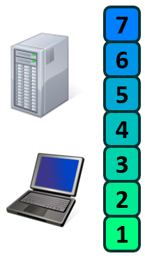
The traditional example would be your computer or laptop. But in these modern times, there are so many more: mobile phones, smart TVs, smart watches, certain cars, and even some refrigerators!
Hosts run software and applications for the end user to interact with, and they also at some point need to put bits on a wire. As such, it is said that Hosts operate across all seven layers of the OSI model.
In typical internet communication or network traffic, the two hosts in communication are often labeled as the Client or the Server.
The Client is the entity initiating the request and is looking to acquire a piece of information or data or a service. While the Server is the entity receiving the request and has the information, data, or service that the Client wants.
It should be noted that these terms are relative to specific types of communication.
For example, when your laptop is browsing through a web page, your laptop is acting as the Client and the Web Server is acting as the Server. But when that same Web Server is then downloading software updates, it is now acting as a Client and communicating with an Update Server.
A Network is simply two or more connected devices — typically grouped together by similar purposes or physical location. A network can take many different forms, for example:
-
A group of PCs in a classroom are all in the same physical space and would all belong to one network.
-
Any typical home network will include multiple laptops, mobile phones, or printers that are all tied to the same physical address. Therefore, all belonging to the same network.
-
A coffee shop which has WiFi will allow each of their customers to connect to the same WiFi Network.
-
A large company might use multiple networks, often separating them by job role. For instance, one network for all its accountants and another network for all its engineers.
Depending on the purpose of each network, the devices within them will then communicate with other devices in the same network or other devices in different networks.
Any time any of the Key Players discussed in this rest of this article series are connected to each other, you have a network. In fact, the whole Internet is nothing more than a series of Inter-connected _net_works.
A Switch is a network device whose primary purpose is to facilitate communication within networks.
Switches operate at Layer 2 of the OSI model, which means they only look into each data-gram up to the Layer 2 header. The Layer 2 header contains information that enables [hop to hop delivery], such as the Source and Destination MAC address.
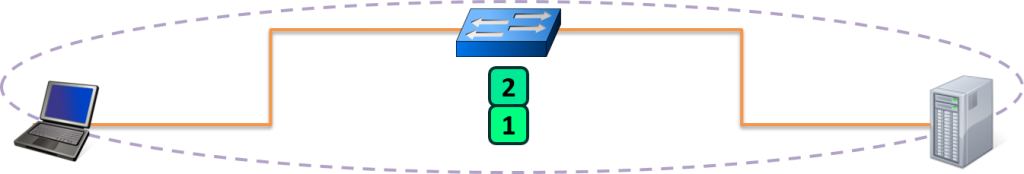
A Switch operates by maintaining what is known as a MAC Address table. This is a table that maps MAC addresses of devices plugged into each switch port. A typical switch has many ports, from 24 to 48, up to 96, or more.
The MAC Address Table is populated by looking at the Source MAC address field of any received frames.
In order to forward the frame, the Switch will lookup the Destination MAC address in their MAC Address Table to determine what port to use.
If a Switch encounters a frame for which it does not know the location of the Destination MAC address, it simply duplicates and floods the frame out each switch port (except the port it was received on). This process will be examined more closely in another article in this series.
A Router is a network device whose primary purpose is to facilitate communication between networks. Each interface on a router creates a network boundary.
Routers operate at Layer 3 of the OSI Model, which means they only look into each datagram up to the Layer 3 header. The Layer 3 header contains information that enables [end to end delivery], such as the Source and Destination IP Address.

In the image above, notice that the router on the left (R1) and the router on the right (R2) create three separate networks (11.11.11.x, 22.22.22.x, and 33.33.33.x). R1’s right interface and R2’s left interface are both on the same network.
The only way for the Client in the 11.11.11.x network to speak to the Server in the 33.33.33.x network is to forward the packet to R1, who will in turn forward the packet to R2, who will then finally forward the packet to the Server.
A Router accomplishes all this by maintaining what is known as a Routing Table. This is a table that contains paths to all the networks a Router knows how to reach. These paths are sometimes known as Routes, and each entry contains an IP Network and either an interface or the IP address of the next router in the path to the target.
There are multiple ways a Router can learn of a network and populate its Routing Table. We will look at some of those ways in a later article in this series.
Keep in mind, from the perspective of each router, the Route Table is a map of every network that exists. If a router receives a packet destined to a network it does not know about, then as far as that router is concerned, that network must not exist. Therefore, when a router receives a packet destined to a network which is not in its Routing Table, that packet is discarded.
Earlier we discussed that MAC addresses are a Layer 2 addressing scheme. We also discussed that IP addresses are a Layer 3 addressing scheme.
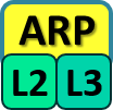
What bridges these two addressing schemes is the Address Resolution Protocol (ARP).
Typically, when two hosts are communicating, they already know each other’s IP address. They can know each other’s IP address from a variety of methods: sometimes it is manually provided by a user, sometimes by another protocol (often DNS). But the actual method employed is irrelevant (at least to this article series).
However, what is definitely not known is their MAC addresses. The hosts will use ARP to discover the appropriate MAC address. To put it another way, ARP will use the known IP address, and discover the unknown MAC address. The discovered mapping is then added and stored in an ARP Table, which is a mapping of IP addresses to correlating MAC addresses.
We’ll describe how L2 and L3 are bridged together, and ARP’s role in the process using the following illustration:

In the image above, there are three networks: the purple network, the gray network, and the red network. We’ll use this diagram to illustrate two instances of ARP: First when a host is speaking to another host in the same network (Client to Purple server). And Second when a host is speaking to another host in a different network (Client to Red server).
When the Client needs to speak to the Purple Server, it will know the Purple Server’s IP address, and from that it will determine that the Purple Server exists in the local network. When a Client is attempting to speak to a host in the same network, the Client will issue an ARP request for the host’s MAC address.
ARP will allow the Client to complete the Layer 2 header as follows:
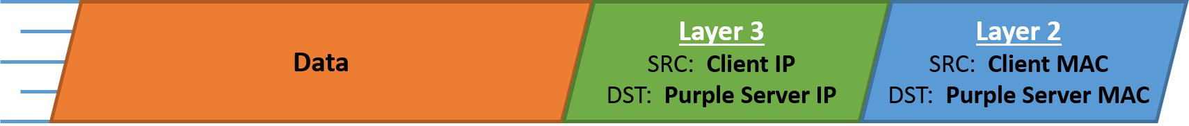
When the Client needs to speak to the Red Server, it will know the Red Server’s IP address, and from that it will know that the Red Server exists in a foreign network. As such, the packet must be delivered to the nearest router — otherwise known as the Default Gateway.
The Client is generally already configured with a Default Gateway — which we can tell from the image will be the R1. When a Client is attempting to speak to a host in a foreign network, the Client will issue an ARP request for the Default Gateway’s MAC address.
This will allow the Client to populate the Layer 3 and Layer 2 headers as follows:
To summarize ARP’s operation:

- When a Client is speaking to a host in the same network, it will ARP for the MAC address of the host
- When a Client is speaking to a host in a different network, it will ARP for the MAC address of the Default Gateway
Remember, packet delivery is always the job of Layer 2, and Layer 2’s primary goal is getting a packet from hop to hop. Conversely, Layer 3, which is concerned with end to end delivery is unable to put a packet on a wire and send it to another host’s NIC. ARP’s role is to help the client create the proper L2 header, based on the L3 header, in order to get the packet from one hop to the next.
It should also be noted that any device that intends to forward a packet based upon the IP address (L3), must also have the ability to deliver the packet to the next hop (L2). As such, any device that uses IP addresses must also use ARP to deliver the packet using MAC addresses. Consequently, all Layer 3 devices must maintain an ARP Table.
For another explanation of ARP and an illustration of the address resolution process in video form, click here.
This article and the [previous] covered a lot of ground on a variety of subjects that individually have entire books written about. This was intentionally done so that the next few articles in the series can bring everything together (and go a bit deeper than this article went). But it is crucial that all the tenants of these two articles be understood before moving forward.
In this article, we discussed the primary purposes of the different layers of the OSI model. Specifically:
- [OSI Layer 1 is the physical medium carrying the 1’s and 0’s across the wire
- [OSI Layer 2 is responsible for hop to hop delivery and uses MAC addresses
- [OSI Layer 3 is responsible for end to end delivery and uses IP Addresses
- [OSI Layer 4 is responsible for service to service delivery and uses Port Numbers
We also discussed some of the Key Players involved in moving a packet through the Internet:
- Switches facilitate communications within networks and operate at Layer 2
- Routers facilitate communication between networks and operate at Layer 3
- ARP uses a known IP address to resolve an unknown MAC address
We also discussed three different tables that are use to store different mappings:
- Switches use a MAC Address Table which is a mapping of Switchports to connected MAC addresses
- Routers use a Routing Table which is a mapping of known Networks to interfaces or next-hop addresses
- All L3 devices use an ARP Table which is a mapping of IP Addresses to MAC addresses
If any of the bullet points above don’t make complete sense, please consider re-reading this article or the one previous before continuing to the next article in this series.
Host to Host Communication
After discussing the makeup of the [OSI Model] and some of the [Key Players] involved in moving a packet from one host to another, we can finally discuss the specific functions which occur in allowing Host to Host communication.
At the very core of the Internet is this idea that two computers can communicate with each other. Although it is rare to find situations where two hosts are connected directly to each other, understanding what happens if they were is crucial to understanding everything else that happens when multiple hosts are communicating through a switch or router.
As such, this article will focus on host to host communication, and each individual step involved in the process.
Since there are no Routers in this illustration, we know all the communication is happening within the same network — therefore, Host A and Host B are both configured with IP addresses that belong to the same network.

Each host has a unique IP address and MAC address. Since each host is also a [L3] device, they each also have an [ARP Table]. At the moment, their ARP Tables are empty.
Host A starts by generating some Data for Host B. Host A knows the final destination for this data will be the IP address 10.10.10.20 (Host B). Host A also knows its own address (10.10.10.10), and as such is able to create a L3 header with the required Source and Destination IP Address.
But as we learned earlier, [packet delivery is the job of Layer 2], so despite these hosts being directly connected to one another, a L2 header must be created.
The Source of the L2 header will be Host A’s MAC address (aaaa.aaaa.aaaa). The Destination of the L2 header should be Host B’s MAC address, but at the moment, Host A doesn’t have an entry in its ARP Table for Host B’s IP address, and therefore, does not know Host B’s MAC address.
As a result, Host A is unable to create the proper L2 header to deliver the packet to Host B’s NIC at this time. Host A will have to initiate an ARP Request in order to acquire the missing information:
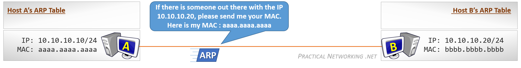
The ARP Request is a single packet which essentially asks: “If there is someone out there with the IP 10.10.10.20, please send me your MAC address.“
Remember, at this point Host A does not know if Host B exists. In fact, Host A does not know that it is directly connected to Host B. Hence, the question is addressed to everyone on the link. The ARP Request is sent as a Broadcast, and had there been other hosts connected to this link, they too would have received the ARP Request.
Also note that Host A includes its own MAC address in the ARP Request itself. This allows Host B (if it exists) to easily respond directly back to Host A with the requested information.
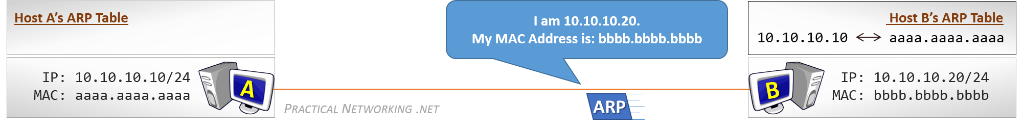
Receiving the ARP Request allows Host B to learn something. Namely, that Host A’s IP address is 10.10.10.10 and the correlating MAC address is aaaa.aaaa.aaaa. Notice this entry is now added to Host B’s ARP Table.
Host B can use this new information to respond directly to Host A. The ARP Response is sent as a Unicast message, directly addressed to Host A. Had there been other hosts on this link, they would not have seen the ARP Response.
The ARP Response will include the information Host A requested: The IP Address 10.10.10.20 is being served by the NIC with the MAC address bbbb.bbbb.bbbb. Host A will use this information to populate its ARP Table:
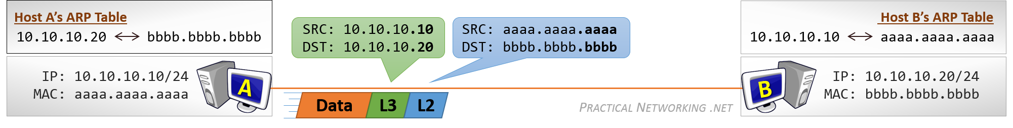
With Host A’s ARP Table populated, Host A can now successfully put together the proper L2 header to get the packet to Host B.
When Host B gets the data, it will be able to respond without further ado, since it already has a mapping in its ARP Table for Host A.
Again, it is rare to find two hosts directly connected to each other. But understanding what it takes to get a packet from one Host to another Host is key to understanding how a Switch enables multi-host communication, or a Router enables multi-network communication. Both of these will be the subjects of the next articles in this series.
The key thing to note is a host doesn’t know whether it is connected to a switch or directly to another host. In either case, the host will follow the process outlined above when trying to communicate with another host.
Interested in learning more about ARP? If so, you might find this video helpful.
In the last article, we looked at everything that happens for two hosts to communicate directly with one another. In this article, we will add a common network device: a switch. We will take a look at what happens for communication from Host to Host through a Switch.
This article will be the practical application of everything that was discussed when we looked at a [Switch] as a key player in packet traveling. It might be worth reviewing that section before proceeding.
We will start by looking at the individual switch functions, and then take a look at an animation which shows their collaborative operation.
A Switch primarily has four functions: Learning, Flooding, Forwarding, and Filtering:
Being a Layer 2 device, a Switch will make all its decisions based upon information found in the L2 Header. Specifically, a Switch will use the Source MAC address and Destination MAC address to make its forwarding decisions.
One of the goals of the Switch is to create a MAC Address Table, mapping each of its switchports to the MAC address of the connected devices.
The MAC address table starts out empty, and every time a Switch receives anything, it takes a look at the Source MAC address field of the incoming frame. It uses the Source MAC and the switchport the frame was received on to build an entry in the MAC Address Table.
Sooner or later, as each connected device inevitably sends something, the Switch will have a fully populated MAC Address Table. This table can then be used to smartly forward frames to their intended destination.
However, despite the learning process above, it is unavoidable that a Switch will at some point receive a frame destined to a MAC address of which the Switch does not know the location.
In such cases, the Switch’s only option is to simply duplicate the frame and send it out all ports. This action is known as Flooding.
Flooding assures that if the intended device exists and if it is connected to the switch, it will definitely receive the frame.
Of course, so will every other device connected to that particular Switch. And though not ideal, this is perfectly normal. The NIC of each connected device will receive the frame and take a look at the Destination MAC address field. If they are not the intended recipient, they will simply silently drop the frame.
If they are the intended device, however, then the Switch can rest satisfied knowing it was able to deliver the frame successfully.
Moreover, when the intended device receives the frame, a response will be generated, which when sent to the Switch will allow the switch to learn and create a MAC Address Table mapping that unknown device to its switchport.
Ideally, of course, the Switch will have an entry in its MAC Address Table for every Destination MAC it comes across.
When this happens, the Switch happily forwards the frame out the appropriate switchport.
There are three methods by which a Switch can forward frames. They are briefly described below.
- Store and Forward – The Switch copies the entire frame (header + data) into a memory buffer and inspects the frame for errors before forwarding it along. This method is the slowest, but allows for the best error detection and additional features like prioritizing certain types of traffic for faster processing.
- Cut-Through – The Switch stores nothing, and inspects only the bare minimum required to read the Destination MAC address and forward the frame. This method is the quickest, but provides no error detection or potential for additional features.
- Fragment Free – This method is a blend of the prior two. The Switch inspects only the first portion of the frame (64 bytes) before forwarding the frame along. If a transmission error occurred, it is typically noticed within the first 64 bytes. As such, this method provides “good enough” error detection, while gaining the speed and efficiency of avoiding storing the entire frame in its memory before forwarding it.
It is worth pointing out that these three methods were at one point very significant when Switch technologies were newer and switching induced noticeable latency. In modern days, with line-speed switching, the difference in speed between these three is negligible, and most switches operate in Store and Forward mode.
And finally, the last function of the switch is filtering. Mainly, this function states that a Switch will never forward a frame back out the same port which received the frame.
Most commonly, this happens when a Switch needs to flood a frame — the frame will get duplicated and sent out every switchport except the switchport which received the frame.
Rarely, a host will send a frame with a destination MAC address of itself. This is usually a host experiencing some sort of error condition or being malicious. Either way, when this happens, the Switch simply discards the frame.
Now that we’ve looked at each of the individual functions of a Switch, we can look at them in action. The animation below includes a Switch going through all four functions as it processes traffic.
Ordinarily, the hosts in the animation below would need to perform an ARP resolution, but for the sake of focusing on the Switch’s operation, we will omit ARP and proceed as if all the hosts already knew each other’s IP and MAC addresses.
Host A has “something” to send to Host B. The contents of the “something” is entirely irrelevant, so long as its understood that the frame has a L2 header which includes a Source and Destination MAC address.
Initially, the MAC Address Table of the Switch is empty. Remember, it only gets populated when a frame is received.
When Host A sends the frame to the switch, it includes a Source MAC address of aaaa.aaaa.aaaa. This prompts the Switch to learn a MAC Address Table entry mapping Port 1 to MAC Address aaaa.aaaa.aaaa.
Then, when deciding how to forward the frame, the Switch realizes there is no entry for bbbb.bbbb.bbbb. This leaves the Switch only one option: duplicate and flood the frame out all ports. Notice the frame was duplicated out all ports, except Port 1 (the port it came in on) – this is an example of the Switch performing its filtering function.
This frame will then be received by Host C and Host B. Host C, when inspecting the L2 header will realize the frame is not intended for them and will simply discard it. Conversely, when Host B receives the frame and realizes they indeed are the intended recipient, they will accept the frame and generate a response.
When the response arrives on the Switch, another MAC Address Table mapping can be learned: Port 2 contains the MAC address bbbb.bbbb.bbbb.
Then the Switch looks up the Destination MAC address (aaaa.aaaa.aaaa) and realizes this address exists out Port 1. The Switch can then simply forward the frame, since it knows the location of the Destination MAC address.
The animation above illustrate the four switch functions on a single switch. To see how the process scales to multiple switches, check out this article.
There is often some confusion about a switch in regards to a Broadcast and a Switch’s flooding behavior. The confusion is understandable, because the end result is the same, but it is also important to understand the distinction.
A Broadcast frame is a frame which is addressed to everyone on the local network. This is done using the same Ethernet header we’ve been discussing, except the Destination MAC address field is populated with a special address: ffff.ffff.ffff. The “all F’s” address is specially reserved for the purpose of broadcasting.
By definition, if the Switch ever encounters a packet with a destination MAC of ffff.ffff.ffff, it will always flood the frame (after learning the Source MAC, of course).
Another way of looking at it, is since the address ffff.ffff.ffff is reserved, the switch is unable to learn a MAC Address Table mapping for it. As such, any frame destined to this MAC address will always be flooded.
In summary, a Broadcast is a frame addressed to everyone on the local network (ffff.ffff.ffff), and Flooding is an action a switch can take. A broadcast frame, by definition, will always be flooded by a switch. But a switch will never broadcast a frame (since broadcasting is not a function of a switch).
This article intentionally omits the Address Resolution Protocol (ARP) in order to focus purely on the actions of a Switch. ARP is a function of the client, and will never be performed by the switch itself. It is assumed that the clients in the animation above already know each other’s MAC address. To learn more about ARP, check out this video.
We’ve looked at what it takes for [two hosts directly connected to each other] to communicate. And we’ve looked at what it takes for a host to speak to another host [through a switch]. Now we add another network device as we look at what it takes for traffic to pass from host to host through a Router.
This article will be the practical application of everything that was discussed when we looked at a [Router] as a key player in Packet Traveling. It might be worth reviewing that section before proceeding.
We will start by looking at the two major Router Functions, then see them in action as we look at Router Operation.
To discuss our way through these concepts, we will use the following image. We will focus on R1, and what is required for it to forward packets from Host A, to Host B and Host C.

For simplicity, the MAC addresses of each NIC will be abbreviated to just four hex digits.
Earlier we mentioned that a Router’s primary purpose is to facilitate communication between networks. As such, every router creates a boundary between two networks, and their main role is to forward packets from one network to the next.
Notice in the image above, we have R1 creating a boundary between the 11.11.11.x network and the 22.22.22.x network. And we have R2 creating a boundary between the 22.22.22.x and 33.33.33.x networks. Both of the routers have an interface in the 22.22.22.x network.
In order to forward packets between networks, a router must perform two functions: populate and maintain a Routing Table, and populate and maintain an ARP Table.
From the perspective of each Router, the Routing Table is the map of all networks in existence. The Routing Table starts empty, and is populated as the Router learns of new routes to each network.
There are multiple ways a Router can learn the routes to each network. We will discuss two of them in this section.
The simplest method is what is known as a Directly Connected route. Essentially, when a Router interface is configured with a particular IP address, the Router will know the Network to which it is directly attached.
For example, in the image above, R1’s left interface is configured with the IP address 11.11.11.1. This tells R1 the location of the 11.11.11.x network exists out its left interface. In the same way, R1 learns that the 22.22.22.x network is located on its right interface.
Of course, a Router can not be directly connected to every network. Notice in the image above, R1 is not connected to 33.33.33.x, but it is very likely it might have to one day forward a packet to that network. Therefore, there must exist another way of learning networks, beyond simply what the router is directly connected to.
That other way is known as a Static Route. A Static Route is a route which is manually configured by an administrator. It would be as if you explicitly told R1 that the 33.33.33.x network exists behind R2, and to get to it, R1 has to send packets to R2’s interface (configured with the IP address 22.22.22.2).
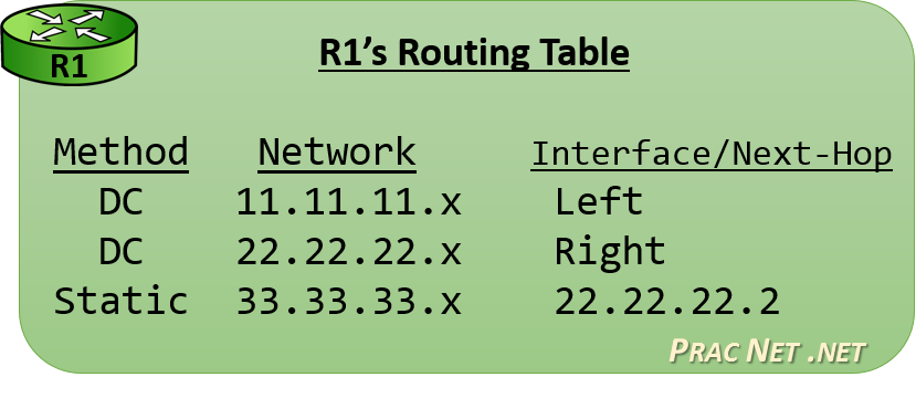
In the end, after R1 learned of the two Directly Connected routes, and after R1 was configured with the one Static Route, R1 would have a Routing Table that looked like this image.
The Routing Table is populated with many Routes. Each Route contains a mapping of Networks to Interfaces or Next-Hop addresses.
Every time a Router receives a packet, it will consult its Routing Table to determine how to forward the packet.
Again, the Routing Table is a map of every network that exists (from the perspective of each router). If a router receives a packet destined to a network it does not have a route for, then as far as that router is concerned, that network must not exist. Therefore, a router will discard a packet if its destination is in a network not in the Routing Table.
Finally, there is a third method for learning routes known as Dynamic Routing. This involves the routers detecting and speaking to one another automatically to inform each other of their known routes. There are various protocols that can be used for Dynamic Routing, each representing different strategies, but alas their intricacies fall outside the scope of this article series. They will undoubtedly become a subject for future articles.
That said, the Routing Table will tell the router which IP address to forward the packet to next. But as we learned earlier, packet delivery is always the job of Layer 2. And in order for the Router to create the L2 Header which will get the packet to the next L3 address, the Router must maintain an [ARP Table].
The [Address Resolution Protocol (ARP)] is the bridge between Layer 3 and Layer 2. When provided with an IP address, ARP resolves the correlating MAC address. Devices employ ARP to populate an ARP Table, or sometimes called an ARP Cache, which is a mapping of IP address to MAC addresses.
A router will use its Routing Table to determine the next IP address which should receive a packet. If the Route indicates the destination exists on a directly connected network, then the “next IP address” is the Destination IP address of the packet – the final hop for that packet.
Either way, the Router will use a L2 header as the vessel to deliver the packet to the correct NIC.

Unlike the Routing Table, the ARP Table is populated ‘as needed’. Which means in the image above, R1 will not initiate an ARP Request for Host B’s MAC address until it has a packet which must be delivered to Host B.
But as we discussed before, an ARP Table is simply a mapping of IP addresses to MAC addresses. When R1’s ARP Table will be fully populated, it will look like this image.
Once again, for simplicity, the images in this article are simply using four hex digits for the MAC addresses. In reality, a MAC address is 12 hex digits long. If its easier, you can simply repeat the four-digit hex MAC address three times, giving R2’s left interface a “real” MAC address of bb22.bb22.bb22.
With the understanding of how a Router populates its Routing Table and how a Router intends to populate its ARP Table, we can now look at how how these two tables are used practically for a Router to facilitate communication between networks.
In R1’s Routing Table above, you can see there are two type of routes: some that point to an Interface, and some that point to a Next-Hop IP address. We’ll frame our discussion around a Router’s operation around these two possibilities.
But first, we will discuss how Host A delivers the packet to its Default Gateway (R1). Then we will look at what R1 does with a packet sent from Host A to Host B, and then another packet that was sent from Host A to Host C.
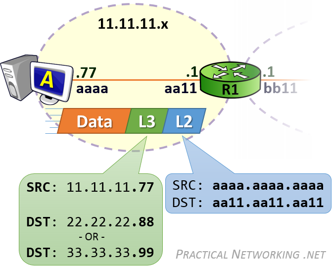
In both cases, Host A is communicating with two hosts on foreign networks. Therefore, Host A will need to get either packet to its default gateway — R1.
Host A will create the L3 header with a Source IP address of 11.11.11.77, and a Destination IP address of 22.22.22.88 (for Host B) or 33.33.33.99 (for Host C). This L3 header will serve the purpose of getting the data from ‘end to end’.
But that L3 header won’t be enough to deliver the packet to R1. Something else (such as MAC) will have to be used.
Host A will then [encapsulate] the L3 header in a L2 header which will include a Source MAC address of aaaa.aaa.aaaa and a Destination MAC address of aa11.aa11.aa11 — the MAC address which identifies R1’s NIC. This L2 header will serve the purpose of delivering the packet across the first hop.
Host A will have already been configured with its Default Gateway’s IP address, and hopefully Host A will have already communicated with foreign hosts. As such, Host A more than likely already had an [ARP Table] entry with R1’s MAC address. Conversely, if this was Host A’s first communication with a foreign host, forming the L2 header would have been preceded with an [ARP Request to discover R1’s MAC address].
At this point, R1 will have the packet. The Destination IP address of the packet will either be 22.22.22.88 for the communication sent to Host B, or 33.33.33.99 for the communication sent to Host C. Both of those destinations exist in [R1’s Routing Table] — the difference is one Route points to an Interface and the other Route points to a Next-Hop IP.
A Route in a Routing Table that points to an Interface was typically learned because the Router was Directly Connected to the network. If a packet’s Destination IP address is in a network which is directly connected to the router, the Router knows they are responsible for delivering the packet to its final hop.
The process is similar to what has been discussed before. The Router uses the L3 header information to determine where to send the packet next, then creates a L2 header to get it there. In this case, the next (and final) hop this packet must take is to the NIC on Host B.

The L3 header will remain unchanged — it is identical to the L3 header created by Host A.
What is different, is the L2 header. Notice the Source MAC address is bb11.bb11.bb11 — R1’s right interface MAC address. The old L2 header which Host A had created to get the packet to R1 was stripped off, and a new L2 header was generated (by R1) to deliver it to the next NIC.
The Destination MAC address is, of course, bbbb.bbbb.bbbb — the MAC address for Host B.
For the packet from Host A sent to Host C, the Destination IP address will be 33.33.33.99. When R1 consults its Routing Table, it will determine that the next-hop for the 33.33.33.x network exists at the IP address 22.22.22.2 — R2’s left interface IP address.
Effectively, this tells R1 to use a L2 header which will get the packet to R2 in order to continue forwarding this packet along its way.
Since the current “hop” is between R1 and R2, their MAC addresses will make up the Source and Destination MAC addresses:
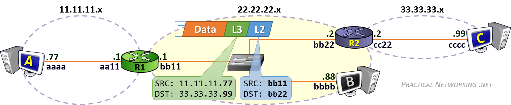
Again, the L3 header remains unchanged, it includes the same Source and Destination IP addresses initially set by Host A — these addresses represent the two “ends” of the communication. The L2 header, however, is completely regenerated at each hop.
Should R1 not have R2’s MAC address, it would simply initiate an ARP Request for the IP address in the route: 22.22.22.2. From then on, it will have no problems creating the proper L2 header which will get the packet from R1 to R2.
As the process continues, R2 will finally receive the packet, and then be faced with the same situation that R1 was in for the example above — deliver the packet to its final hop.
This process can be continued as needed. Had Host A been trying to speak to Host X which had 10 routers in the path, the process would have been identical. Each transit Router in the path would have a Route mapping Host X’s network to the next-hop IP in the path. Until the final router which would be directly connected to the network Host X resided in. And that final router would be responsible for delivering the packet to its final hop — Host X itself.
In this series, we studied the different layers of the [OSI Model], and how each of the seven layers provides a unique service which the other layers depend on.
We also studied the [key players] of the Internet, where we defined a [Host], [Client]), [Server], [Switch], [Router], and [ARP]. As well as each of their unique roles in moving a packet its path.
We then looked at the specific workings of a [Switch], and its exact functions as it facilitates communication within a network. Then we looked at the specific workings of a [Router], and exactly how it facilitates communication between networks.
Finally, its time to finish the [Packet Traveling series] with a video that ties everything together. In the following video, we will look at everything that happens to get data from Host A to Host D, as it passes from a Host, through a Switch, to a Router, through another Switch, and finally to its final destination.

Communication through Multiple Switches
In a previous article we demonstrated [how a single switch functions]. One of the most frequent requests I receive is asking how the process would be different if there were multiple switches. This article will illustrate the process using two switches.
In the [Packet Traveling series], we discussed the four specific functions of a switch: [Learning], [Flooding], [Forwarding], and [Filtering]; we then illustrated each function in an animation that showed [two hosts communicating through a single switch].
With multiple switches, each switch will still independently perform the exact same four functions. The process does not change, it is simply replicated separately by other switches.
We will illustrate how data moves between multiple switches using the following topology:
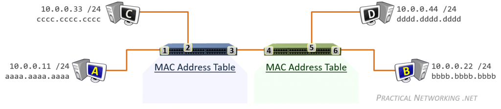
Our topology has two switches, and each has their own, independent MAC address table — the information in the MAC address tables are never shared.
Host A and C are connected to ports 1 and 2 of the blue switch on the left. Host B and D are connected to ports 5 and 6 of the green switch on the right. Port 3 on the blue switch is connected to port 4 on the green switch.
We will illustrate each step that occurs for each of the following:
- Initial frame from Host A to Host B
- Response from Host B to Host A
- Continued communication between Host A and Host B
It starts with Host A having a frame to deliver to Host B. The contents of the frame are irrelevant, it could be an ICMP (ping) packet, it could be an ARP packet, or it could be other data.
The Layer3 header would include a Source IP address of 10.0.0.11 (Host A) and a Destination IP address of 10.0.0.22 (Host B).
The Layer2 header would include a Source MAC address of aaaa.aaaa.aaaa and a Destination MAC address of bbbb.bbbb.bbbb. The switches will use the information in the Layer2 header to move the frame between the two hosts.
To begin, the MAC address tables for both switches will be empty. They will populate as the switches [learn] of each device connected to each port by reading the Source MAC address field of each received frame.
When the frame arrives on the blue switch, the first thing that happens is the blue switch [learns] the MAC address aaaa.aaaa.aaaa exists on port 1. Then, since the blue switch does not yet have an entry in tis MAC address table for bbbb.bbbb.bbbb, the frame is duplicated and [flooded] out every port.
The frame arrives on Host C, who will inspect the frame and realize it is not the intended recipient. Host C will silently discard the frame.
The frame will also arrive on the green switch. Just like the other switch, the first thing the green switch will do is [learn] that it received a frame on port 4 with a source MAC address of aaaa.aaaa.aaaa. And again, just like the other switch, the green switch does not know where the MAC address bbbb.bbbb.bbbb exists, so the frame will again be duplicated and [flooded] out each switch port.
Notice in both cases, the frame was flooded out each port, except the port it was received on. This is an example of a switch’s [filtering] behavior. This behavior prevents a switch from sending a frame out the same port it was received.
Host D will receive the frame, and silently discard it since the frame was not addressed to Host D.
Host B will receive the frame and accept it for processing, since Host B was the intended destination..
On the way back things will go a little simpler. The switches have already learned about some of the connected devices, and that should alleviate some of the additional flooding that was required for the initial communication in the previous section.
Specifically, both switches know the location of the MAC address aaaa.aaaa.aaaa – port 1 on the blue switch and port 4 on the green switch. Each switch learned the location independent of the other; there was no communication between the switches or sharing of MAC address tables.
In the response frame sent by Host B to Host A, the Layer2 header will have a Source MAC address of bbbb.bbbb.bbbb and a Destination MAC address of aaaa.aaaa.aaaa.
The response frame will first arrive on the green switch on port 6. Therefore, the green switch will learn that the MAC address bbbb.bbbb.bbbb exists out port 6. The green switch then consults its MAC address table to determine that the frame destined to aaaa.aaaa.aaaa should be [forwarded] out port 4.
The response frame then arrives on the blue switch on port 3. Therefore, the blue switch will learn the MAC address bbbb.bbbb.bbbb exists out port 3. The blue switch then consults its MAC address table to determine that the frame destined to aaaa.aaa.aaaa should be [forwarded] out port 1.
Which will finally get the response frame back to Host A. Notice on the way back no flooding was required. Both switches knew the location of the destination MAC address of the frame.
Finally, with the both switches’ MAC address tables fully populated, communication between Host A and Host B resembles the following:
Each time a frame is received, the switch first attempts to learn the MAC address mapping on the receiving switch port. If the mapping is already known, it is simply refreshed in the MAC address table.
Notice, Host C and D receive none of the frames sent between Host A and B. The switch is able to create an isolated path for the data between these two hosts (so long as the MAC address tables remain populated).
This is one of the benefits of upgrading to a Switch from a simple Hub. With a Hub, every frame is flooded out every port, every time. Whereas with a switch (or a “smart hub”, as they are sometimes referred to) only the first few frames will be flooded, but all remaining communication between two hosts is confined to only those two hosts.
At some point in time, all hosts will have sent some frames, providing both switches the opportunity to learn the location of each MAC address in the topology above. At that point, the switch MAC address tables will resemble the image below:
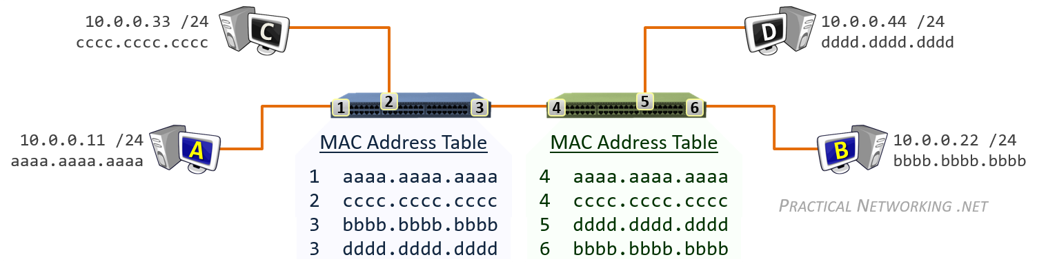
The key item to note is that each switch port can learn of multiple MAC addresses. Notice, from the blue switch’s perspective, the location of Host B and D is out port 3. Moreover, from the green switch’s perspective, the location of host A and Host C is out port 4.
Below is the entire process of Host A and Host B communicating, from beginning to end, and including the ability to pause/forward/rewind the animation. If you’ve read through this article and understand each step described above, you can use this animation to study. Or even better, to explain the process to someone else.
If the animation above did not load, try this link
https://www.practicalnetworking.net/index/vlans-index/
The following index of articles all cover various aspects of Virtual Local Area Networks, or VLANs. They are listed here in one place to make it easier to find if you are interested in learning more about VLANs.
This handy shortlink has been created which will always take you to this page:
Practical Networking – VLAN articles:
- Virtual Local Area Networks (VLANs)
- VLANs (above article, but in Video format)
- Configuring VLANs on Cisco switches
- Routing Between VLANs
- What is the Native VLAN?
- Voice VLAN — Auxiliary VLAN
Virtual Local Area Networks, or VLANs, are a very simple concept that has been very poorly defined by the industry.
This article will explain VLANs from a practical perspective. It will be framed around the two major functions of VLANs, and concluded with an explanation of the idea behind the Native VLAN.
Finally, at the end of the article is a two question comprehension challenge – if you can successfully answer these two questions, then you can consider yourself to fully understand the concept of VLANs — the topic of [configuring VLANs] will be covered in another article.
Below is a network with three different physical switches. The [switches facilitate communication within networks], and the [Routers facilitate communication between networks].
Each switch above independently perform all the functions of a switch.
If each of these switches have 24 ports and only two are in use, then 22 ports are left wasted on each switch. Moreover, what if you need to replicate this network elsewhere and you do not have three physical switches to accommodate?
That is where the first major function of a VLAN comes into play: A VLAN allows you to take one physical switch, and break it up into smaller mini-switches.
Consider each circle on the switch below as its own mini-switch (or virtual switch). Each of these mini-switches are a collection of switch ports which operate completely independent from the others — exactly as they would had there been three different physical switches.
Traffic flow through the single switch of this topology operates exactly as it did in the topology above it with three separate physical switches. The routers are configured and operate exactly as they did above.
Each virtual switch, or VLAN, is simply a number assigned to each switch port. For example, the two switch ports in the red mini-switch might be assigned to VLAN #10. The two ports in the orange mini-switch might be assigned to VLAN #20. And lastly the two switch ports in the blue mini-switch might be assigned to VLAN #30.
Any switch port which is not explicitly assigned a VLAN number, resides in the default VLAN. Which for most vendors corresponds to VLAN 1.
Traffic arriving on a switch port assigned to one VLAN will only ever be forwarded out another switch port that belongs to the same VLAN – a switch will never allow traffic to cross a VLAN boundary. Again, each VLAN operates as if it were a completely separate physical switch.
In the [first illustration], traffic from the red switch cannot magically appear on the orange switch without first passing through a router. Similarly, in the [second illustration], traffic in VLAN #10 cannot magically appear on VLAN #20 without also [passing through a router].
When a frame arrives on a switchport in VLAN #10, it can only leave a switchport in VLAN #10. You and I can see that the same frame is traversing all three VLANs, but from the Switch’s perspective, it is three different instances of a frame arriving on one port in one VLAN, and leaving on another port in the same VLAN.
By definition, a Switch is a device whose primary [purpose is to move data within IP Networks]. To accomplish this goal, every switch maintains a [MAC Address Table], which is a mapping of the MAC addresses connected to every Switchport. A simple representation of a single entry in a MAC address table would be: MAC Address | Port.
A Switch which supports VLANs will also include the VLAN # for each entry of the MAC Address Table. A simple representation of a single entry in a MAC address table of a VLAN aware switch would be: VLAN# | MAC Address | Port.
In a way, it’s almost as if each VLAN maintains their own independent MAC address table. If Host A were to send a frame with a destination MAC address of Host B, that frame would still only be flooded solely to the switch ports in VLAN #10. Even if a MAC address table entry for Host B existed associated to VLAN #30.
Ultimately, assigning different ports to different VLANs allows you to re-use a single physical switch for multiple purposes. This is the first major function of a VLAN.
But that isn’t all VLANs allow you to do. The second major function is VLANs allow you to extend the smaller Virtual switches across multiple Physical switches.
To illustrate this point, we will expand the topology above with an additional physical switch and two additional hosts:
Notice how a VLAN# 10 and VLAN# 30 have been extended onto a second switch. This enables Host A and Host C to exist in the same VLAN, despite being connected to different physical switches located in potentially different areas.
The primary benefit of extending a VLAN to different physical switches is that the Layer 2 topology no longer has to be tied to the Physical Topology. A single VLAN can span across multiple rooms, floors, or office buildings.
Each connected switch port in the topology above is a member of only a single VLAN. This is referred to as an Access port. An Access port is a switch port that is a member of only one VLAN.
When configuring a port as an Access port, the administrator also designates the VLAN number that port is a member of. Whenever the switch receives any traffic on an Access port, it accepts the traffic onto the configured VLAN.
In order to extend a VLAN to the second switch, a connection is made between one Access port on both switches for each VLAN. While functional, this strategy does not scale. Imagine if our topology was using ten VLANs, on a 24 port switch nearly half of the ports would be taken up by the inter-switch links.
Instead, there is a mechanism which allows a single switch port to carry traffic from multiple VLANs. This is referred to as a Trunk port. A Trunk port is a switch port that carries traffic for multiple VLANs.
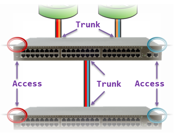
We can use Trunk ports to reduce the amount of switch ports required for the topology above. This enables us to leave more ports available to add hosts to the network in the future.
This physical topology operates (logically) identically to the illustration above it, but requires far fewer switch ports.
We were able to use a total of four Trunk ports (across both switches) to replace eight different Access ports in the prior illustration.
Typically, switch ports connected to end-host devices are configured as Access ports (e.g., workstations, printers, servers). Conversely, switch ports connected to other network devices are configured as Trunk ports (e.g., other switches, routers). We will uncover the reason for this later in this article.
A Trunk port on a switch can receive traffic for more than one VLAN. For example, in the illustration above, the link between the two switches is carrying traffic for both VLAN 10 and VLAN 30.
But in both cases, traffic is leaving one switch as a series of frames, and arriving on the other switch as a series of frames. Which begs the question, how will the receiving switch determine which frames belong to VLAN #10, and which frames belong to VLAN #30?
To account for this, whenever a Switch is sending frames out a Trunk port, it adds to each frame a tag to indicate to the other end what VLAN that frame belongs to. This allows the receiving switch to read the VLAN tag in order to determine what VLAN the incoming traffic should be associated to.
An Access port, by comparison, can only ever carry or receive traffic for a single VLAN. Therefore, there is no need to add a VLAN Tag to traffic leaving an Access port.
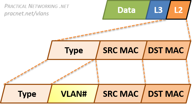
Since VLANs are a Layer 2 technology, the VLAN Tag is inserted within the Layer 2 header. The standard Layer 2 header in modern networks is the Ethernet header, which has three fields: Destination MAC Address, Source MAC Address, and Type.
When an Ethernet frame is exiting a Trunk port, the switch will insert a VLAN Tag between the Source MAC address and the Type fields.
This allows the receiving switch to associate the frame with the appropriate VLAN.
To summarize, the final topology with traffic traveling between Host C and Host D through Access ports and Trunk ports will look like this:
The physical topology above will work exactly like the logical topology below. The hosts will not know whether they are going through two physical switches ([or three or four]), or what VLANs they are in. They operate exactly as they would in any situation which involves moving packets through a network.

Earlier we mentioned Access ports typically face end-host devices like workstations or printers or servers.
Part of the reason for this is that [switches do not add a VLAN tag when sending traffic out an Access Port].
This allows a host to operate without any knowledge of the VLAN they are connected to.
In a way, the hosts are, intentionally, completely blind to the existence or use of VLANs. Hosts simply send data on a network without any knowledge of VLANs, or the switches they might be connected to.
There was a point in the early days of Networking where certain end-devices would react negatively if they received a frame with a VLAN tag. For such systems, which were strictly expecting only the typical fields in an Ethernet header, the frames which included a VLAN tag might appear as a malformed Ethernet header.
However, this was rare, as the construction of the VLAN tag was intentionally designed to avoid being interpreted as a malformed frame (this will make more sense in the next section).
Either way, the general precedent is traffic to end-hosts should not include any VLAN tags, Hosts can and should remain blissfully ignorant of what VLANs they are in, or even whether VLANs are being utilized at all.
A possible exception would be if a single Physical Host is hosting multiple Virtual Machines (VMs) — like a Hypervisor. In some cases, each of those VMs need to exist in separate VLANs. Therefore, the Physical Host must be connected to a Trunk port, and must send and received VLAN tags in order to confine the virtual machine traffic to a specific VLAN.
Finally, a quick note on terminology. The terms Access port and Trunk port are usually associated with the Cisco world. But VLANs are an open standard, therefore other vendors are able to implement VLANs as well.
What Cisco calls a Trunk port (i.e., a switch port that carries traffic for more than one VLAN), other vendors refer to as a Tagged port – referring to the addition of a VLAN tag to all traffic leaving such a port.
What Cisco calls an Access port (i.e., a switch port that carries traffic for only one VLAN), other vendors refer to as an Untagged port – referring to the traffic leaving the switch port without a VLAN tag.
These terms are not exhaustive, there are some vendors that may yet use other terminology, other vendors may even mix and match these terms. Regardless of the terminology used, all the concepts discussed above still apply.
VLAN tags requires adding and removing bits to Ethernet frames. The specific sequence of bits to add is governed by an open standard, which allow any vendor to implement VLANs on their devices.
The exact format of the VLAN Tag is governed by the 802.1Q standard. This is an open, IEEE standard which is the ubiquitous method of VLAN tagging in use today.
To demonstrate exactly how the VLAN Tag modifies a packet, take a look at the packet capture below of the same frame before and after it exits a Trunk port.
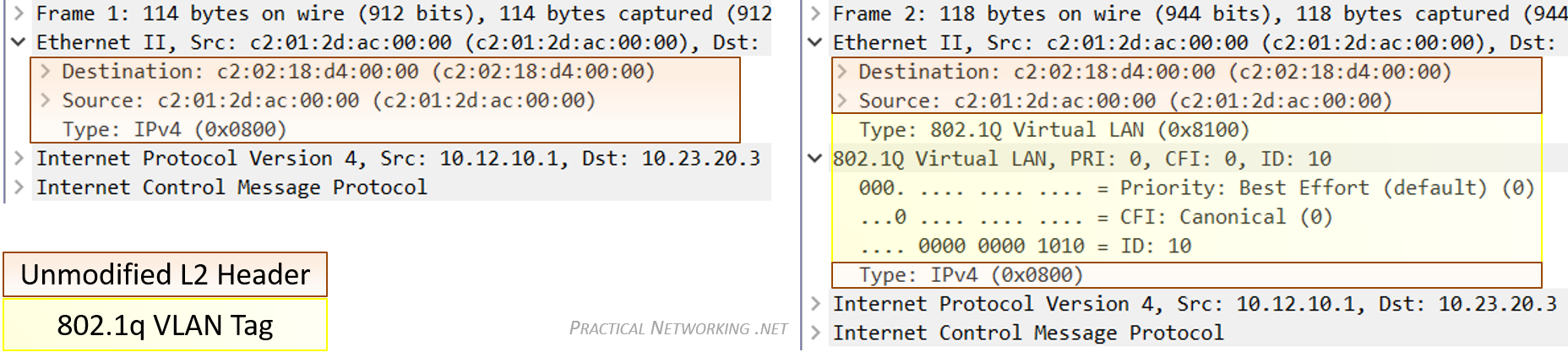
The portion of the frame highlighted in yellow is the added VLAN tag. Notice it is inserted between the Source MAC address and Type field of the original Ethernet header.
You can view this capture yourself in Cloudshark, or you can download the capture file and open it in Wireshark.
No other modification to the frame or its payload is made by the addition or removal of the VLAN tag. That said, since even the slight modification displayed above is made, adding and removing the VLAN tag also involves recalculating the CRC — which is a simple hash algorithm devised to detect transmissions errors on the wire.
There is an older method of VLAN tagging which is a closed, Cisco proprietary method. This method was called Inter-Switch Link, or ISL. ISL fully [encapsulated] the L2 frame in a new header which included the VLAN identification number.
But these days, even newer Cisco products do not support ISL, as the entire industry has moved to the superior, open standard of 802.1Q.
There is one final concept associated with VLANs that often brings confusion. That is the concept of the Native VLAN.
The Native VLAN is the answer to how a switch processes traffic it receives on a Trunk port which does not contain a VLAN Tag.
Without the tag, the switch will not know what VLAN the traffic belongs to, therefore the switch associates the untagged traffic with what is configured as the Native VLAN. Essentially, the Native VLAN is the VLAN that any received untagged traffic gets assigned to on a Trunk port.
Additionally, any traffic the switch forwards out a Trunk port that is associated with the Native VLAN is forwarded without a VLAN Tag.
To see the Native VLAN in action on a live trunk port, check out this video.
The Native VLAN can be configured on any Trunk port. If the Native VLAN is not explicitly designated on a Trunk port, the default configuration of VLAN #1 is used.
That being said, it is crucially important that both sides of a Trunk port are configured with the same Native VLAN. This illustration explains why:
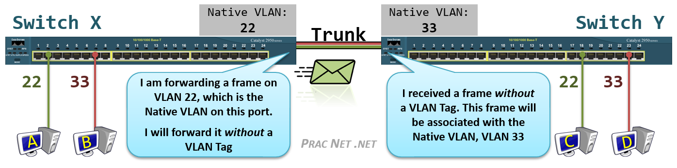
Above we have four Hosts (A, B, C, D) all connected to Access Ports in VLAN #22 or VLAN #33, and Switch X and Switch Y connected to each other with a Trunk port.
Host A is attempting to send a frame to Host C. When it arrives on the switch, Switch X associates the traffic with VLAN #22. When the frame is forwarded out Switch X’s Trunk port, no tag is added since the Native VLAN for the Trunk Port on Switch X is also VLAN #22.
But when the frame arrives on Switch Y without a tag, Switch Y has no way of knowing the traffic should belong to VLAN #22. All it can do is associate the untagged traffic with what Switch Y’s Trunk port has configured as the Native VLAN, which in this case is VLAN #33.
Since Switch Y will never allow VLAN #33 traffic to exit a VLAN #22 port, Host C will never get this traffic. Even worse, due to a Switch’s [flooding] behavior, Host D might inadvertently get the traffic that was destined to Host C.
Finally, it should be noted that the Native VLAN is an 802.1Q feature. The antiquated tagging mechanism of ISL simply dropped traffic receive on a Trunk port that did not include the ISL tag. Also, remember that the Native VLAN concept only applies to Trunk ports — traffic leaving and arriving on an Access port is always expected to be untagged.
To test yourself to see if you fully understand how VLANs work, there is a simple challenge we can offer.
Below is a (poorly) configured topology, featuring five switches and twelve hosts. Each switch port is configured as either an Access port in the displayed VLAN, or a Trunk Port with the Native VLAN displayed.
The challenge is to answer just these two simple questions:
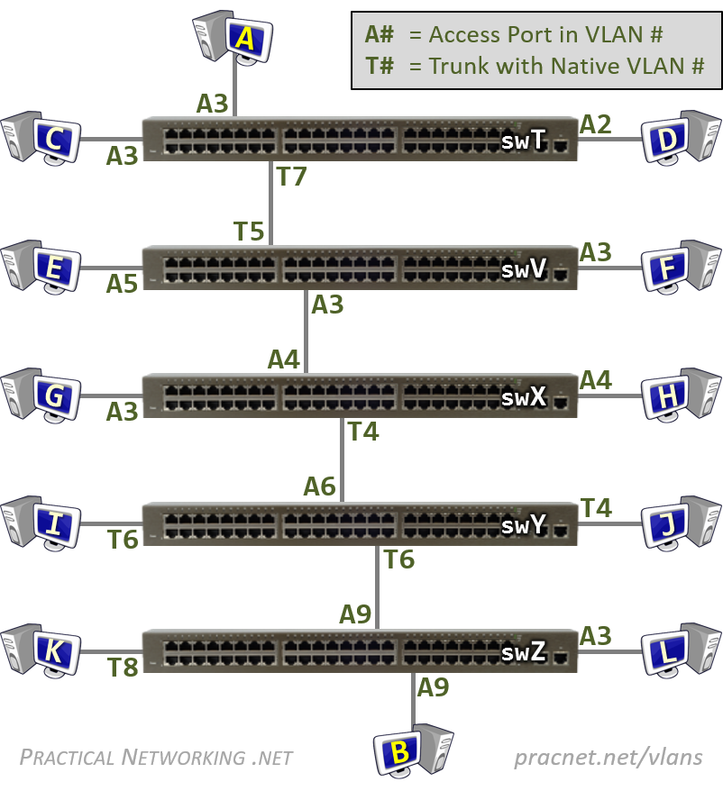
Question #1:
If Host A sends a frame to Host B, will Host B receive it?
Question #2:
If Host A sends a Broadcast, which hosts will receive it?
Answer to Question #1
Yes, Host B will receive the frame that Host A sends.
To understand why, you will need to have a solid understanding of when a Switch sends a frame [tagged or untagged], and what a switch does when it receives a frame that is tagged or untagged.
We will step through the sequence of events to prove it. For this answer, we are only going to focus on the connection above and below each switch, and not the connections that are left and right (i.e., ignoring the connections to Host C through Host L).
It starts with Host A sending the frame untagged since hosts do not understand VLAN tags, nor do they know what VLAN is configured on the switch port they are connected to.
Switch T receives the untagged frame on an Access Port in VLAN #3. Switch T therefore considers the frame to be in VLAN #3. The port below Switch T is a Trunk port, which means all traffic leaving the port must have a VLAN tag. Except for traffic on the Native VLAN, which in this case is VLAN #7 – not the VLAN that our frame is on. Therefore, the frame leaves Switch T tagged for VLAN #3.
Switch V receives the tagged frame and reads the tag to determine the frame belongs to VLAN #3. Switch V then forwards the frame untagged out the Access Port in VLAN #3 — all traffic leaving an Access port is untagged.
Switch X receives the untagged frame on an Access Port in VLAN #4. Since there is no tag, Switch X associates the frame to VLAN #4. Switch X then forwards the frame out the Trunk port, but since this Trunk port has a Native VLAN of VLAN #4, the frame is sent untagged.
Switch Y receives the untagged frame on an Access Port in VLAN #6. Switch Y now considers the frame to be in VLAN #6. Switch Y then forwards the frame out a Trunk port, but since this Trunk port has a Native VLAN of VLAN #6, the frame is sent untagged.
Switch Z receives the untagged frame on an Access Port in VLAN #9. Switch Z now considers the frame to be in VLAN #9. Switch Z then forwards the frame out an Access port – which is always sent untagged.
Host B then finally, successfully, receives the untagged frame.
Answer to Question #2
The following hosts will receive a broadcast frame sent from Host A:
C, F, H, I, B
Note: Host J and Host K also receive the broadcast, but when they receive the frame, it will include a VLAN tag. Some hosts are able to receive frames with VLAN tags, and some hosts are not — it depends on whether the host understands 802.1q VLAN tags.
To explain this answer, you must first fully understand Question #1 and its answer. Once you have fully grasped why a frame from Host A is able to get to Host B, you can then try to understand Question #2 and the explanation below.
The key is to determine what VLAN# each switch will consider the broadcast frame to be a part of. From there, you can easily determine whether the hosts to the left or right will receive the frame. We already know from Question #1 that what is sent by Host A will make its way through each switch in the topology, so all there is to consider is whether the other hosts will receive it.
Again, it starts with Host A sending the frame untagged to Switch T.
Switch T considers the frame in VLAN #3. Therefore, it does forward the broadcast out the Access port in VLAN #3, and does NOT forward the frame out the Access port in VLAN #2. Host C receives it, Host D does not.
Switch V considers the frame in VLAN #3. Therefore, it does NOT forward the broadcast out the Access port in VLAN #5, and does forward the broadcast out the Access port in VLAN #3. Host E does not receive the frame, Host F does.
Switch X considers the frame in VLAN #4. Therefore, it does NOT forward the broadcast out the Access port in VLAN #3, and does forward the broadcast out the Access port in VLAN #4. Host G does not receive the frame, Host H does.
Switch Y considers the frame in VLAN #6. It does forward the frame out both Trunk ports. However, if the Trunk port is configured with a Native VLAN that matches the frame, then the frame is sent untagged. Therefore, when Host I receives the frame, it receives the frame without a VLAN tag and is able to understand the L2 header. When Host J receives the frame, it includes a VLAN tag. Host I is able to receive and process the frame as normal, but Host J is only able to receive the frame if Host J supports 802.1q VLAN tags.
Switch Z considers the frame in VLAN #9. It does forward the frame out the Trunk port with Native VLAN #8, but it does so with a VLAN Tag. Host K can only process the frame if Host K understands 802.1q VLAN tags. Switch Z does NOT forward the frame out the Access Port in VLAN #3, therefore Host L never receives the broadcast frame.
Finally, since we’ve already answered the first question, we know Host B will receive a frame that Host A sends.
The topology above is constructed purely to test your understanding of a frame flowing through switches, passing through Tagged and Untagged ports. It is decidedly a very bad Layer 2 design and should not be considered for any real deployments. It is merely a teaching tool. =)
Routing Between VLANs & Layer 3 Switches
We wrote an article which covers [Virtual Local Area Networks (VLANs)] as a concept, and another article on [configuring VLANs on Cisco switches]. The remaining subjects to cover are the different options that exist for routing between VLANs. This will let us illustrate the concepts of inter-vlan routing, Router on a Stick (RoaS), and Layer 3 Switches (occasionally called MultiLayer Switches).
As we learned in a prior article, VLANs create a [logical separation] between Switch ports. Essentially, each VLAN behaves like a separate physical switch. To illustrate this, below are two topology pictures of the same environment – one Physical and one Logical.
The Physical topology depicts a switch and four hosts in two different VLANs – Host A and Host B are in VLAN 20 and Host C and Host D are in VLAN 30. The logical topology reflects how the physical topology operates – the two VLANs essentially create two separate physical switches.
Physical vs. Logical
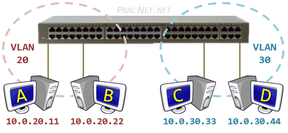
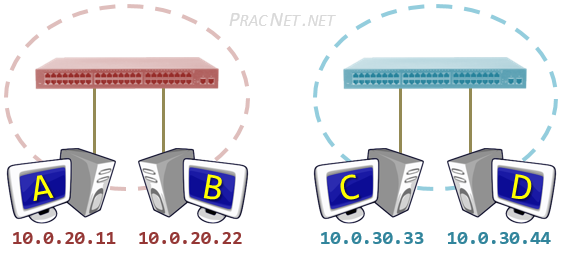
Despite all four hosts being connected to the same physical switch, the logical topology makes it clear that the hosts in VLAN 20 are unable to speak with the hosts in VLAN 30. Notice since there is nothing connecting the two “virtual” switches, there is no way for Host A to speak to Host C.
Since Host A and Host C are in different VLANs, it is also implied that they are in different Networks. Each VLAN will typically correspond to its own [IP Network]. In this diagram, VLAN 20 contains the 10.0.20.0/24 network, and VLAN 30 contains the 10.0.30.0/24 network.
The purpose of a Switch is to facilitate communication within networks. This works great for Host A trying to speak to Host B. However, if Host A is trying to speak to Host C, we will need to use another device – one whose purpose is to facilitate communication between networks.
If you’ve read the [Packet Traveling] series, then you know that the device which facilitates communication between networks is a [Router].
A router will perform the routing function necessary for two hosts on different networks to speak to one another. In the same way, a Router is what we will need in order for hosts in different VLANs to communicate with one another.
There are three options available in order to enable routing between the VLANs:
- Router with a Separate Physical Interface in each VLAN
- Router with a Sub-Interface in each VLAN
- Utilizing a Layer 3 Switch
The remainder of this article will explore these three options and their configuration.
The simplest way to enable routing between the two VLANs to simply connect an additional port from each VLAN into a Router.

The Router doesn’t know that it has two connections to the same switch — nor does it need to. The Router operates like normal when routing packets between two networks.
In fact, the process of a packet moving from Host A to Host D in this topology will work exactly as it does in this video. The only difference is since there is only one physical switch, there will only be one MAC address table – each entry includes the mapping of switchport to MAC address, as well as the VLAN ID number that port belongs to.
Each switch port in this diagram is configured as an [Access port], we can use the range command to configure multiple ports as once:
Switch(config)# **interface range eth2/0 - 2**
Switch(config-if-range)# **switchport mode access**
Switch(config-if-range)# **switchport access vlan 20**

Switch(config)# **interface range eth3/0 - 2**
Switch(config-if-range)# **switchport mode access**
Switch(config-if-range)# **switchport access vlan 30**
Of course, before [assigning the switchport to a VLAN], it is a good idea to [create the VLAN in the VLAN Database].
The Router interfaces also use a standard configuration — configuring an IP address and enabling the interface:
Router(config)# **interface eth0/2**
Router(config-if)# **ip address 10.0.20.1 255.255.255.0**
Router(config-if)# no shutdown

Router(config)# **interface eth0/3**
Router(config-if)# **ip address 10.0.30.1 255.255.255.0**
Router(config-if)# no shutdown
Below you will find various show commands for the Router and the Switch, these can be used to understand and validate how the environment is functioning.
- show running-config
- show ip interface brief
- show ip route
- show arp
- show cdp neighbors
Router# show running-config
...
interface Ethernet0/2
 ip address 10.0.20.1 255.255.255.0
!
interface Ethernet0/3
 ip address 10.0.30.1 255.255.255.0


Router# show ip interface brief
Interface             IP-Address      OK? Method Status        Protocol
...
**Ethernet0/2           10.0.20.1**       YES manual up            up
**Ethernet0/3           10.0.30.1**       YES manual up            up
...


Router# show ip route
Codes: L - local, C - connected, ...

Gateway of last resort is not set

      10.0.0.0/8 is variably subnetted, 4 subnets, 2 masks
C        **10.0.20.0/24 is directly connected, Ethernet0/2**
L        10.0.20.1/32 is directly connected, Ethernet0/2
C        **10.0.30.0/24 is directly connected, Ethernet0/3**
L        10.0.30.1/32 is directly connected, Ethernet0/3


Router# show arp
Protocol  Address          Age (min)  Hardware Addr   Type   Interface
Internet  10.0.20.1               -   aabb.cc00.0220  ARPA   Ethernet0/2
Internet  **10.0.20.11**              2   **0050.7966.6800**  ARPA   **Ethernet0/2**
Internet  **10.0.20.22**              5   **0050.7966.6801**  ARPA   **Ethernet0/2**
Internet  10.0.30.1               -   aabb.cc00.0230  ARPA   Ethernet0/3
Internet  **10.0.30.33**              4   **0050.7966.6802**  ARPA   **Ethernet0/3**
Internet  **10.0.30.44**              4   **0050.7966.6803**  ARPA   **Ethernet0/3**


Router# show cdp neighbors
Capability Codes: R - Router, S - Switch, I - IGMP, B - Source Route Bridge
...
Device ID        Local Intrfce     Holdtme    Capability  Platform  Port ID
**Switch           Eth 0/3**           126             R S I  Linux Uni Eth 3/0
**Switch Eth 0/2** 126 R S I Linux Uni Eth 2/0- show running-config
- show mac address-table
- show vlan brief
- show cdp neighbors
Switch# show running-config
...
vlan 20
 name RED
!
vlan 30
 name BLUE
...
interface Ethernet2/0
 switchport access vlan 20
 switchport mode access
!
interface Ethernet2/1
 switchport access vlan 20
 switchport mode access
!
interface Ethernet2/2
 switchport access vlan 20
 switchport mode access
!
interface Ethernet3/0
 switchport access vlan 30
 switchport mode access
!
interface Ethernet3/1
 switchport access vlan 30
 switchport mode access
!
interface Ethernet3/2
 switchport access vlan 30
 switchport mode access


Switch# show mac address-table
          Mac Address Table
-------------------------------------------

Vlan    Mac Address       Type        Ports
----    -----------       --------    -----
  20    0050.7966.6800    DYNAMIC     Et2/1
  20    0050.7966.6801    DYNAMIC     Et2/2
  20    aabb.cc00.0220    DYNAMIC     Et2/0
  30    0050.7966.6802    DYNAMIC     Et3/1
  30    0050.7966.6803    DYNAMIC     Et3/2
  30    aabb.cc00.0230    DYNAMIC     Et3/0
Total Mac Addresses for this criterion: 6


Switch# show vlan brief

VLAN Name                        Status    Ports
---- --------------------------- --------- --------------------
...
**20   RED**                         active    **Et2/0, Et2/1, Et2/2**
**30   BLUE**                        active    **Et3/0, Et3/1, Et3/2**
...


Switch# show cdp neighbors
Capability Codes: R - Router, S - Switch, I - IGMP, B - Source Route Bridge
...
Device ID        Local Intrfce     Holdtme    Capability  Platform  Port ID
**Router           Eth 3/0**           152              R B   Linux Uni Eth 0/3
**Router Eth 2/0** 166 R B Linux Uni Eth 0/2The previously described method is functional, but scales poorly. If there were five VLANs on the switch, then we would need five switchports and five router ports to enable routing between all five VLANs
Instead, there exists a way for multiple VLANs to terminate on a single router interface. That method is to create a Sub-Interface.
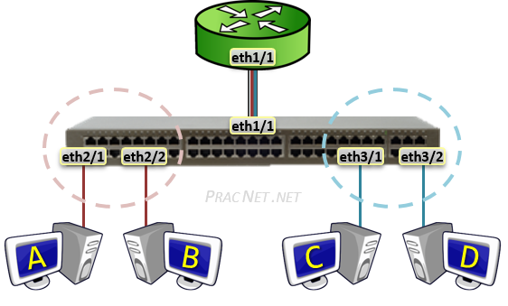
A Sub-Interface allows a single Physical interface to be split up into multiple virtual sub-interfaces, each of which terminate their own VLAN.
Sub-interfaces to a Router are similar to what [Trunk ports] are to a Switch – one link carrying traffic for multiple VLANs. Hence, each router Sub-interface must also add a [VLAN tag] to all traffic leaving said interface.
The logical operation of the Sub-interface topology works exactly as the separate physical interface topology in the section before it. The only difference is with Sub-interfaces, only one Router interface is required to terminate all VLANs.
Keep in mind, however, that the drawback with all VLANs terminating on a single Router interface is an increased risk of congestion on the link.
The Sub-interface feature is sometimes referred to as Router on a Stick or One-armed Router. This is in reference to the single router terminating the traffic from each VLAN.
The Switch’s port facing the router is configured as a standard Trunk:
Switch(config)# interface eth1/1
Switch(config-if)# switchport trunk encapsulation dot1q
Switch(config-if)# switchport mode trunk
The Router’s configuration of Sub-interfaces is fairly straight forward. First, we enable the physical interface:
Router(config)# interface eth1/1
Router(config-if)# no shutdown
Next, we create and configure the first Sub-interface:
Router(config)# interface eth1/1.20
Router(config-subif)# encapsulation dot1Q 20
Router(config-subif)# ip address 10.0.20.1 255.255.255.0
Apart from using the Sub-interface distinguisher (eth1/1**.20**) and using the encapsulation dot1q <VLAN#> command, the rest of the interface configuration is exactly the same as any other regular [physical interface].
Similarly, we will also configure the Sub-interface for VLAN 30:
Router(config)# interface eth1/1.30
Router(config-subif)# encapsulation dot1Q 30
Router(config-subif)# ip address 10.0.30.1 255.255.255.0
A point of clarity regarding the Sub-interface syntax. The number after the physical interface (fa0/3.20 and fa0/3.30) simply serves the purpose of splitting up the physical interfaces into Sub-interfaces. The number specified in the encapsulation dot1q vlan ## command is what actually specifies what VLAN ID# the traffic belongs to.
These two values do not have to match, but often they do for the purpose of technician sanity.
Below you will find various show commands for the Router and the Switch. These can be used to understand and validate how the environment is functioning.
- show running-config
- show ip interface brief
- show ip route
- show arp
- show cdp neighbors
Router# show running-config
...
interface Ethernet1/1
 no ip address
!
**interface Ethernet1/1.20
 encapsulation dot1Q 20
 ip address 10.0.20.1 255.255.255.0**
!
**interface Ethernet1/1.30
 encapsulation dot1Q 30
 ip address 10.0.30.1 255.255.255.0**


Router# show ip interface brief
Interface             IP-Address      OK? Method Status        Protocol
...
Ethernet1/1           unassigned      YES NVRAM  up            up
**Ethernet1/1.20        10.0.20.1**       YES manual up            up
**Ethernet1/1.30        10.0.30.1**       YES manual up            up
...


Router# show ip route
Codes: L - local, C - connected, ...

Gateway of last resort is not set

      10.0.0.0/8 is variably subnetted, 4 subnets, 2 masks
C        **10.0.20.0/24 is directly connected, Ethernet1/1.20**
L        10.0.20.1/32 is directly connected, Ethernet1/1.20
C        **10.0.30.0/24 is directly connected, Ethernet1/1.30**
L        10.0.30.1/32 is directly connected, Ethernet1/1.30


Router# show arp
Protocol  Address          Age (min)  Hardware Addr   Type   Interface
Internet  10.0.20.1               -   aabb.cc00.0211  ARPA   Ethernet1/1.20
Internet  **10.0.20.11**              0   **0050.7966.6800**  ARPA   **Ethernet1/1.20**
Internet  **10.0.20.22**              0   **0050.7966.6801**  ARPA   **Ethernet1/1.20**
Internet  10.0.30.1               -   aabb.cc00.0211  ARPA   Ethernet1/1.30
Internet  **10.0.30.33**              0   **0050.7966.6802**  ARPA   **Ethernet1/1.30**
Internet  **10.0.30.44**              0   **0050.7966.6803**  ARPA   **Ethernet1/1.30**


Router# show cdp neighbors
Capability Codes: R - Router, S - Switch, I - IGMP, B - Source Route Bridge
...
Device ID        Local Intrfce     Holdtme    Capability  Platform  Port ID
**Switch Eth 1/1** 150 R S I Linux Uni Eth 1/1- show running-config
- show mac address-table
- show vlan brief
- show interfaces trunk
- show cdp neighbors
Switch# show running-config
...
vlan 20
 name RED
!
vlan 30
 name BLUE
...
**interface Ethernet1/1
 switchport trunk encapsulation dot1q
 switchport mode trunk**
!
interface Ethernet2/1
 switchport access vlan 20
 switchport mode access
!
interface Ethernet2/2
 switchport access vlan 20
 switchport mode access
!
interface Ethernet3/1
 switchport access vlan 30
 switchport mode access
!
interface Ethernet3/2
 switchport access vlan 30
 switchport mode access


Switch# show mac address-table
          Mac Address Table
-------------------------------------------

Vlan    Mac Address       Type        Ports
----    -----------       --------    -----
   1    aabb.cc00.0211    DYNAMIC     Et1/1
  20    aabb.cc00.0211    DYNAMIC     Et1/1
  30    aabb.cc00.0211    DYNAMIC     Et1/1
  20    0050.7966.6800    DYNAMIC     Et2/1
  20    0050.7966.6801    DYNAMIC     Et2/2
  30    0050.7966.6802    DYNAMIC     Et3/1
  30    0050.7966.6803    DYNAMIC     Et3/2
Total Mac Addresses for this criterion: 7


Switch# show vlan brief

VLAN Name                        Status    Ports
---- --------------------------- --------- -------------------
...
**20   RED**                         active    **Et2/1, Et2/2**
**30   BLUE**                        active    **Et3/1, Et3/2**
...


Switch# show interfaces trunk

Port        Mode             Encapsulation  Status        Native vlan
**Et1/1       on               802.1q         trunking**      1

Port        Vlans allowed on trunk
Et1/1       1-4094

Port        Vlans allowed and active in management domain
**Et1/1**       1,**20,30**

Port        Vlans in spanning tree forwarding state and not pruned
Et1/1       1,20,30


Switch# show cdp neighbors
Capability Codes: R - Router, S - Switch, I - IGMP, B - Source Route Bridge
...
Device ID        Local Intrfce     Holdtme    Capability  Platform  Port ID
**Router Eth 1/1** 136 R B Linux Uni Eth 1/1The last option for routing between VLANs does not involve a router at all. Nor does it involve using a traditional switch.
Instead, a different device entirely can be used. This device is known as a Layer 3 Switch (or sometimes also as a Multilayer switch). But exactly what is a Layer 3 switch?

A Layer 3 Switch is different from a traditional Layer 2 Switch in that it has the functionality for routing between VLANs intrinsically. In fact, when considering how a L3 Switch operates, you can safely imagine that a Layer 3 Switch is a traditional switch with a built in Router.
With regard to VLANs the Multilayer switch is configured mostly the same way as a regular L2 switch:
**MultilayerSwitch**(config)# vlan 20
**MultilayerSwitch**(config-vlan)# name RED
**MultilayerSwitch**(config)# vlan 30
**MultilayerSwitch**(config-vlan)# name BLUE

**MultilayerSwitch**(config)# interface range eth2/0 - 2
**MultilayerSwitch**(config-if-range)# switchport mode access
**MultilayerSwitch**(config-if-range)# switchport access vlan 20

**MultilayerSwitch**(config)# interface range eth3/0 - 2
**MultilayerSwitch**(config-if-range)# switchport mode access
**MultilayerSwitch**(config-if-range)# switchport access vlan 30
Then, for each VLAN that you want the Multilayer switch to route for, you have the option of configuring an IP address within what is known as an SVI, or a Switched Virtual Interface.
An SVI serves as the L3 termination point for each VLAN – aka, the way in or out of each VLAN. Another way of looking at it is that the SVI serves as the interface on the built-in Router of the Multilayer switch, allowing traffic from one VLAN to reach the built-in Router and be routed to another VLAN as necessary.
The configuration for an SVI involves two parts. First, enabling IP Routing; and Second, applying an IP address to the VLAN.
To enable IP Routing, use the following command:
MultilayerSwitch(config)# **ip routing**IP Routing only needs to be enabled once. Some L3 switches come with it enabled by default. Applying the command while it is already enabled will not cause any harm, so if in doubt as to whether it is already enabled or not, simply applying it again is safe.
To apply an IP address to the VLANs, configure the SVI as follows:
MultilayerSwitch(config)# **interface vlan 20**
MultilayerSwitch(config-if)# **ip address 10.0.20.1 255.255.255.0**
MultilayerSwitch(config-if)# no shutdown

MultilayerSwitch(config)# **interface vlan 30**
MultilayerSwitch(config-if)# **ip address 10.0.30.1 255.255.255.0**
MultilayerSwitch(config-if)# no shutdown
The two configurations above will enable routing between VLAN 20 and VLAN 30. The hosts in each VLAN can use the IP addresses 10.0.20.1 and 10.0.30.1 as their default gateway (respectively).
When Host A sends a packet to Host B, the packet will be switched within the same VLAN – no L3 processing will occur.
When Host A sends a packet to Host C, the packet will be sent to the SVI to be routed to the other VLAN – all regular L3 processing will occur: the TTL will be decremented and [the L2 header will be rewritten].
- show running-config
- show mac address-table
- show vlan brief
MultilayerSwitch# show running-config
...
**ip routing**
...
**interface Vlan20
 ip address 10.0.20.1 255.255.255.0**
!
**interface Vlan30
 ip address 10.0.30.1 255.255.255.0**


MultilayerSwitch# show mac address-table
          Mac Address Table
-------------------------------------------

Vlan    Mac Address       Type        Ports
----    -----------       --------    -----
  20    0050.7966.6800    DYNAMIC     Et2/1
  20    0050.7966.6801    DYNAMIC     Et2/2
  30    0050.7966.6802    DYNAMIC     Et3/2
  30    0050.7966.6803    DYNAMIC     Et3/1
Total Mac Addresses for this criterion: 4


MultilayerSwitch# show vlan brief

VLAN Name                        Status    Ports
---- --------------------------- --------- -------------------
...
**20   RED**                         active    **Et2/1, Et2/2**
**30 BLUE** active **Et3/1, Et3/2**- show ip route
- show arp
- show ip interface brief
MultilayerSwitch# show ip route
Codes: L - local, C – connected, ...

Gateway of last resort is not set

      10.0.0.0/8 is variably subnetted, 4 subnets, 2 masks
**C        10.0.20.0/24 is directly connected, Vlan20**
L        10.0.20.1/32 is directly connected, Vlan20
**C        10.0.30.0/24 is directly connected, Vlan30**
L        10.0.30.1/32 is directly connected, Vlan30


MultilayerSwitch# show arp
Protocol  Address          Age (min)  Hardware Addr   Type   Interface
Internet  10.0.20.1               -   aabb.cc80.0200  ARPA   Vlan20
Internet  **10.0.20.11**              0   **0050.7966.6800**  ARPA   **Vlan20**
Internet  **10.0.20.22**              0   **0050.7966.6801**  ARPA   **Vlan20**
Internet  10.0.30.1               -   aabb.cc80.0200  ARPA   Vlan30
Internet  **10.0.30.33**              0   **0050.7966.6803**  ARPA   **Vlan30**
Internet  **10.0.30.44**              0   **0050.7966.6802**  ARPA   **Vlan30**


MultilayerSwitch# show ip interface brief
Interface         IP-Address      OK? Method Status        Protocol
...
**Ethernet2/1       unassigned**      YES unset  up            up
**Ethernet2/2       unassigned**      YES unset  up            up
...
**Ethernet3/1       unassigned**      YES unset  up            up
**Ethernet3/2       unassigned**      YES unset  up            up
...
**Vlan20            10.0.20.1**       YES manual up            up
**Vlan30            10.0.30.1**       YES manual up            up
Note: both sets of tabs and configuration above are from the same device. For the sake of organization, one set of tabs refer to the L3 functions and the other refers to the L2 functions.
This article discussed the three different options for Routing between VLANs. In each case, the hosts in communication behave exactly the same. In fact, the hosts have no visibility into how and what they are connected to.
Each strategy above has its own benefits and limitations. Hopefully at this point you have a good idea of the options available to enable communication between hosts on different VLANs.
https://www.practicalnetworking.net/stand-alone/vpn-overlapping-networks/
When connecting two sites together using a Virtual Private Network (VPN), a common issue that is encountered is trying to build a VPN with overlapping networks — where both sites happen to use the same Private IP addresses.
In such cases, hosts on one side of the VPN tunnel will be unable to communicate with the hosts on the other.
The problem can be circumvented, however, with clever use of Network Address Translation.
In the example below, there are two sites – Seattle and Denver – connected with a VPN tunnel between R1 and R2. Both Seattle and Denver are using 10.0.0.0/24 for their internal network.
Host A in Seattle (10.0.0.77) needs to speak to Host D in Denver (10.0.0.88).
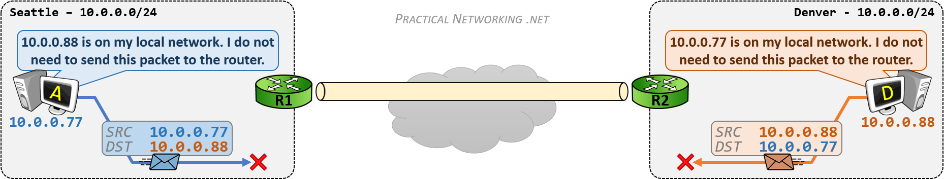
Since Host A is configured with the IP 10.0.0.77/24, Host A believes that every IP address in the range of 10.0.0.0 – 10.0.0.255 exists on its own local network in Seattle. Therefore, if Host A attempts to send a packet to 10.0.0.88, it [will not send the packet to the Router].
Host D will have the same problem, Host D is configured with the IP 10.0.0.88/24 and also believes that the range 10.0.0.0 – 10.0.0.255 exists on its own local network in Denver. Therefore, any packet Host D sends to the IP 10.0.0.77 will be sent to the local network, and not to the Router.
If the packets are not sent to the Router, then the Routers are unable to forward them through the VPN tunnel to the other side. As a result, because of the overlapping networks, neither side will be able to speak to the other.
The solution to the problem is to convince each host that the other host is on a foreign network. That would cause them to send packets to the Router, which can then send them through the VPN tunnel.
This will be attained by making the Seattle network appear as 10.1.1.0/24 when speaking to Denver, and making the Denver network appear as 10.2.2.0/24 when speaking to Seattle.
There are two ways of deploying [Network Address Translation] to facilitate this solution, one involves a NAT configuration on both routers, the other a NAT configuration on one router.
This article uses Routers as the device’s performing NAT. Many other devices can also perform NAT and the concepts described will still apply.
The first solution involves using [Policy NAT] on both routers to mask their internal network when speaking to the opposite side. Recall that a Policy NAT is a type of NAT that involves [making a translation decision based upon matching both the source and destination address].
R1’s Policy NAT configuration will match packets with a Source IP of 10.0.0.0/24 (Seattle’s actual network) and a Destination IP of 10.2.2.0/24 (Denver’s masked network), and translate the Source IP to the 10.1.1.0/24 network (Seattle’s masked network).
R2’s Policy NAT configuration will match packets with a Source IP of 10.0.0.0/24 (Denver’s actual network) and a Destination IP of 10.1.1.0/24 (Seattle’s masked network), and translate the Source IP to the 10.2.2.0/24 network (Denver’s masked network).
In this way, R1 is masking the Seattle 10.0.0.0/24 network as 10.1.1.0/24, and R2 is masking the Denver 10.0.0.0/24 network as 10.2.2.0/24.
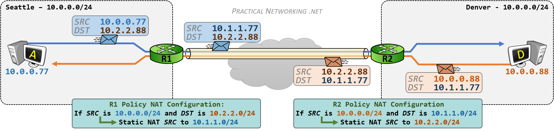
When Host A sends a packet to Host D, the source IP will be 10.0.0.77 and the destination IP will be 10.2.2.88 – an IP address in a foreign network. Host A will send this packet to R1, who will change the Source IP to 10.1.1.77 in accordance with R1’s Policy NAT configuration.
The same will occur when Host D sends a packet to Host A – the packet will have a source of 10.0.0.88 and a destination of 10.1.1.77. This packet will be sent to R2, who will translate the source IP to 10.2.2.88.
Inside the VPN tunnel, the packets will be appear as if the 10.1.1.x network is speaking to the 10.2.2.x network.
When each hosts’ packet arrives at the opposite router, the router will un-translate the destination address back to the appropriate IP address:
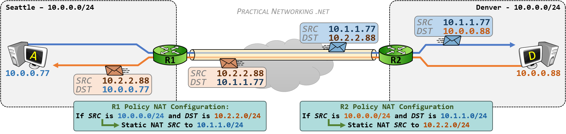
R2 will un-translate the destination IP of the blue packet from 10.2.2.88 to 10.0.0.88 and send the packet to Host D.
R1 will un-translate the destination IP of the red packet from 10.1.1.77 to 10.0.0.77 and send the packet to Host A.
This will enable hosts in Seattle and hosts in Denver to speak to each other, despite both sites having IP addresses in overlapping networks.
The whole process can be seen in the illustration below. This is, essentially, a combination of both images above, with the translations each router is responsible for highlighted:
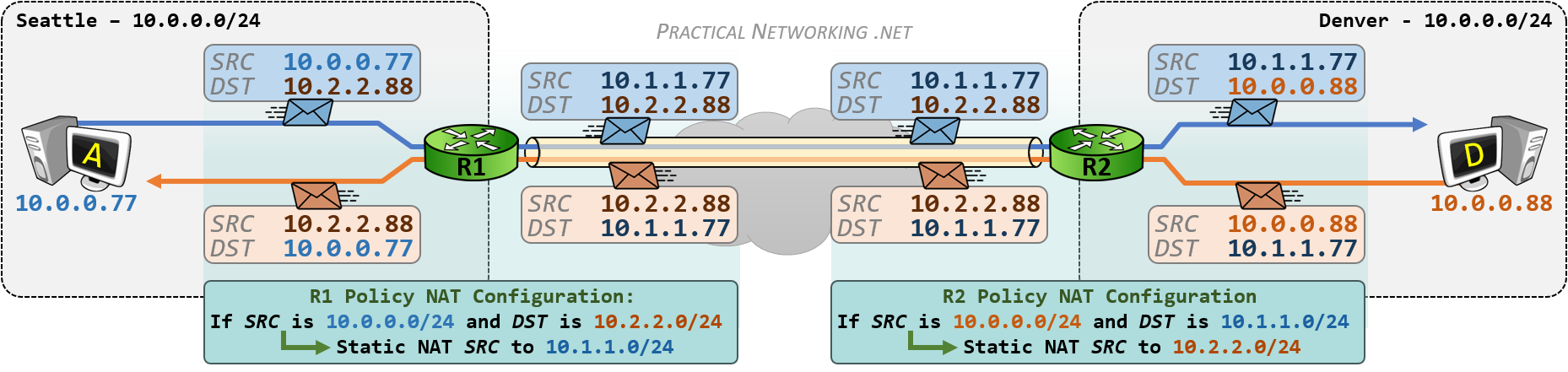
Solution #1 requires both Routers to configure a Policy NAT. However, there are times when the NAT Device on one side does not support a Policy NAT configuration. In those cases, all the address translation will have to occur on a single device. Which brings us to Solution #2.
Solution #2 will still involve a [Policy NAT] – making a NAT decision based upon the Source and Destination. In addition, Solution #2 will also involve a [Twice NAT] – translating both the Source and Destination. Combined, Solution #2 will require [Policy Twice NAT] configuration.
Solution #2 will still solve the overlapping networks problem in the same way – by convincing the local site that the opposite site is on a foreign network. The only difference is Solution #2 will attain this effect by deploying address translation on only one router.
Once again, the goal will be to make the Seattle network appear as 10.1.1.0/24 when speaking to Denver, and make the Denver network appear as 10.2.2.0/24 when speaking to Seattle.
Since Host A (in Seattle) considers Denver as 10.2.2.0/24, R1 must be configured with a Policy NAT that matches traffic with a Source of 10.0.0.0/24 and a destination of 10.2.2.0/24.
For matched traffic, the source will be translated from 10.0.0.0/24 to 10.1.1.0/24 (making Seattle appear as the 10.1.1.0/24 network). Additionally, the destination will be translated from 10.2.2.0/24 to 10.0.0.0/24 (to allow the packet’s to be successfully delivered to Denver’s true network).
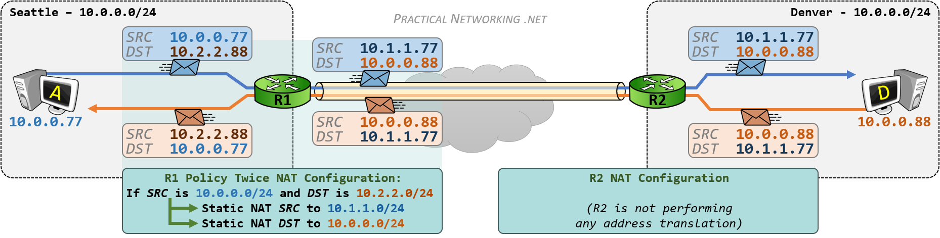
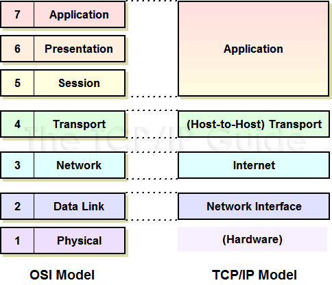
On the way back, when Host D is responding, the packet will have a source of 10.0.0.88 and a destination of 10.1.1.77. The packet will be sent to R2, which will forward it through the VPN tunnel. Upon arriving at R1, R1 will un-translate the packet:
The source IP of 10.0.0.88 will be translated to 10.2.2.88 (making Denver appear as the 10.2.2.0/24 network), and the destination IP of 10.1.1.77 will be translated to 10.0.0.77 (to allow the response packet to be successfully delivered to Seattle’s true network).
In this way, we can use a single Policy Twice NAT on one side of the VPN tunnel to mimic the behavior of using a Policy NAT on both sides outlined in [Solution #1].
In the end, both solutions above accomplished the same goal: they made it seem like the IP networks on either side of the VPN tunnel were unique, and did not overlap.
Of course, the ideal situation would be for both sides of the VPN tunnel to actually have unique IP networks. But failing that, the solutions above provide a practical work around.
Comparing the two solutions, [Solution #1] is cleaner, and most likely to lend itself to simpler troubleshooting and debugging in the future. Both sides of the VPN tunnel are equally contributing to the overall solution.
[Solution #2], while viable, should be reserved only for cases where both sides are unable to or unwilling to configure a Policy NAT.
Either way, solving the problem of overlapping networks on a VPN simply involves using two tools in the Network Address Translation arsenal: Policy NAT and Twice NAT.