scTenifoldNet

A R/MATLAB package to construct and compare single-cell gene regulatory networks (scGRNs) using single-cell RNA-seq (scRNA-seq) data sets collected from different conditions based on machine learning methods. scTenifoldNet uses principal component regression, tensor decomposition, and manifold alignment, to accurately identify even subtly shifted gene expression programs.

Install:

scTenifoldNet requires numpy and scipy from the Python programming language, to install them, we recommend to install miniconda Python: https://docs.conda.io/en/latest/miniconda.html.

After install the Phyton dependencies, install scTenifoldNet, using the following command:

library(devtools)
install_github('cailab-tamu/scTenifoldNet')
library(scTenifoldNet)

Available functions:

Code	Function
installPyDependencies	Install the Phyton dependencies using the reticulate package
scQC	Performs single-cell data quality control
cpmNormalization	Performs counts per million (CPM) data normalization
pcNet	Computes a gene regulatory network based on principal component regression
makeNetworks	Computes gene regulatory networks for subsamples of cells based on principal component regression
tensorDecomposition	Performs CANDECOMP/PARAFAC (CP) Tensor Decomposition
manifoldAlignment	Performs non-linear manifold alignment of two gene regulatory networks
dCoexpression	Evaluates gene differential coexpression based on manifold alignment distances
scTenifoldNet	Gonstruct and compare single-cell gene regulatory networks (scGRNs) using single-cell RNA-seq (scRNA-seq) data sets collected from different conditions based on principal component regression, tensor decomposition, and manifold alignment.

Example:

Loading scTenifoldNet

Once installed, scTenifoldNet can be loaded typing:

library(scTenifoldNet)

Simulating of a dataset

Here we simulate a dataset of 2000 cells (columns) and 100 genes (rows) following the negative binomial distribution with high sparsity (~67%). We label the last ten genes as mitochondrial genes ('mt-') to perform single-cell quality control.

nCells = 2000
nGenes = 100
set.seed(1)
X <- rnbinom(n = nGenes * nCells, size = 20, prob = 0.98)
X <- round(X)
X <- matrix(X, ncol = nCells)
rownames(X) <- c(paste0('ng', 1:90), paste0('mt-', 1:10))

Generating a perturbed network

We generate a perturbed network modifying the expression of genes 10, 2, and 3 and replacing them with the expression of genes 50, 11, and 5.

Y <- X
Y[10,] <- Y[50,]
Y[2,] <- Y[11,]
Y[3,] <- Y[5,]

scTenifoldNet

Here we run scTenifoldNet under the H0 (there is no change in the coexpression profiles) using the same matrix as input and under the HA (there is a change in the coexpression profiles of some genes) using the control and the perturbed network.

outputH0 <- scTenifoldNet(X = X, Y = X,
                          nc_nNet = 10, nc_nCells = 500,
                          td_K = 3, qc_minLibSize = 30,
                          dc_minDist = 0)

outputHA <- scTenifoldNet(X = X, Y = Y,
                          nc_nNet = 10, nc_nCells = 500,
                          td_K = 3, qc_minLibSize = 30,
                          dc_minDist = 0)

Differential coexpression based on manifold alignment distances

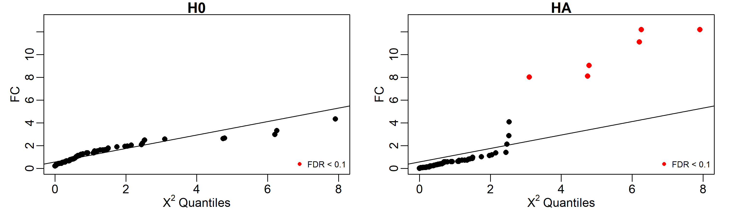
As is shown below, under the H0, none of the genes shown a significative difference in coexpression profiles using an FDR cut-off of 0.1, but under the HA, the 6 genes involved in the perturbation (50, 11, 2, 10, 5, and 3) are identified as perturbed.

head(outputH0$diffCoexpression, n = 10)
#    gene     distance        Z    p.value     p.adj
# 23 ng23 3.070131e-15 2.321093 0.01014092 0.5925054
# 2   ng2 3.028738e-15 2.261954 0.01185011 0.5925054
# 19 ng19 2.912207e-15 2.093459 0.01815409 0.6051362
# 34 ng34 2.769999e-15 1.883624 0.02980793 0.7227582
# 9   ng9 2.617076e-15 1.652429 0.04922353 0.7227582
# 79 ng79 2.602655e-15 1.630314 0.05151755 0.7227582
# 61 ng61 2.582711e-15 1.599635 0.05483975 0.7227582
# 71 ng71 2.489774e-15 1.455239 0.07280162 0.7227582
# 20 ng20 2.479350e-15 1.438890 0.07509082 0.7227582
# 16 ng16 2.461000e-15 1.410037 0.07926437 0.7227582

head(outputHA$diffCoexpression, n = 10)
#    gene   distance        Z     p.value      p.adj
# 50 ng50 0.03122694 3.016417 0.001278908 0.05348371
# 11 ng11 0.03027085 2.955685 0.001559876 0.05348371
# 2   ng2 0.03013548 2.946972 0.001604511 0.05348371
# 10 ng10 0.02759308 2.777666 0.002737543 0.06065138
# 5   ng5 0.02657637 2.706716 0.003397617 0.06065138
# 3   ng3 0.02625458 2.683841 0.003639083 0.06065138
# 31 ng31 0.01309219 1.490124 0.068095790 0.92871127
# 96 mt-6 0.01099588 1.223016 0.110661811 0.92871127
# 6   ng6 0.01067100 1.178311 0.119336356 0.92871127
# 59 ng59 0.01063989 1.173978 0.120201927 0.92871127

Plotting the results

Results can be easily displayed using quantile-quantile plots. Here we labeled in red the identified perturbed genes with FDR < 0.1.

par(mfrow=c(1,2), mar=c(3,3,1,1), mgp=c(1.5,0.5,0))
geneColor <- ifelse(outputH0$diffCoexpression$p.adj < 0.1, 'red', 'black')
qqnorm(outputH0$diffCoexpression$Z, pch = 16, main = 'H0', col = geneColor)
qqline(outputH0$diffCoexpression$Z)
legend('bottomright', legend = c('FDR < 0.1'), pch = 16, col = 'red', bty='n', cex = 0.7)

geneColor <- ifelse(outputHA$diffCoexpression$p.adj < 0.1, 'red', 'black')
qqnorm(outputHA$diffCoexpression$Z, pch = 16, main = 'HA', col = geneColor)
qqline(outputHA$diffCoexpression$Z)
legend('bottomright', legend = c('FDR < 0.1'), pch = 16, col = 'red', bty='n', cex = 0.7)