Subquery

Background

Subquery is frequently used in SQL and introduces considerable complexity.

It can be executed directly as a sub-plan by replacing its correlated column with outer value. The performance is bad because the execution is repeated for each outer row.

Most databases introduce some "unnesting" techniques to unnest the subquery, and convert it to normal join(semi join, anti join, left join, etc).

Here is an example:

SELECT c0 FROM t0 WHERE EXISTS (SELECT 1 FROM t1 WHERE t0.c1 = t1.c1)

The unnested plan is simple:

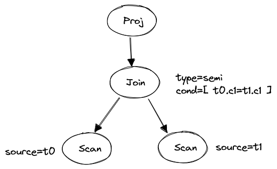
Figure 1. Unnest subquery

There are canonical rules for such "IN", "EXISTS" unnesting, but a little tricky for "NOT IN" due to null handling and existence check on empty set.

But that is not enough. We may have subqueries with join or union, with disjunctive conditions, with conditional evaluation, with nested subqueries. Is there any global rule that can handle most cases?

Formula

The primary formula is:

T1 ⧑(p) T2 = T1 ⨝(p∧T1=𝛢(D))(D⧑T2)) where D := Π(ϝ(T2)∩𝛢(T1))(T1)).

With this formula, we can unnest almost any subquery with following steps:

1. Convert subquery to dependent join, suppose outer table is R, inner query is S.
2. Build a duplicate-free table D from R, including keys in R and correlated columns in S.
3. Construct dependent join T for D and S.
4. Convert T to a normal join T'.
5. Join R and T'.

After above steps, we've converted the subquery to a 3-way join.

The better thing is, in many cases intermediate table can be eliminated for free and leave us just one normal join, reducing the complexity from O(n*m) to O(n), assume we have hash implementation for the logical join.

Note: The "dependent join" is mentioned in original paper, and it has another well-known name: apply operator. In subsequent chapters, I will use "apply" to refer to it.

See details of the formula in paper "Unnesting Arbitrary Queries".

Case Analysis

Now let's classify and analyze subqueries. After that we will discuss how to implement unnesting for majority of those cases.

Non-correlated scalar subquery

SELECT (SELECT count(*) FROM t1)
FROM t2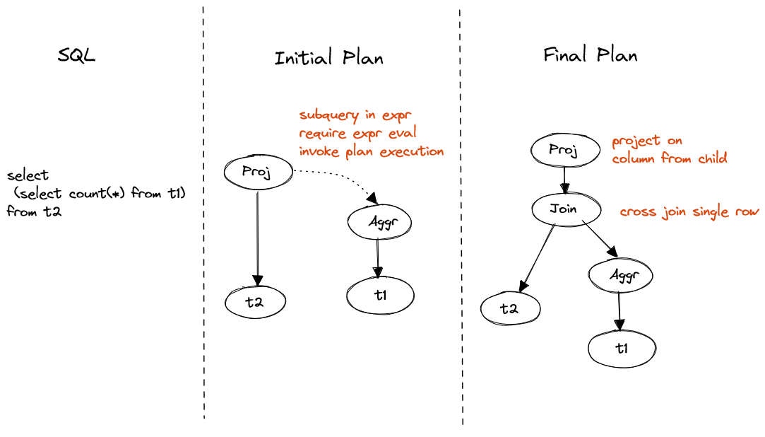

Figure 2. Non-correlated scalar subquery

Non-correlated subquery can be represented as a value cross join on single row.

Value cross join

Value cross join is a specialized cross join that requires right side is scalar value (single row, single column). Differing it from common corss join enables optimizer to have more flexibility of operator reordering.

It also applies to non-correlated scalar subquery in selection and join condition.

Correlated scalar subquery

SELECT (SELECT c0 FROM t1 WHERE t1.c1 = t2.c1)
FROM t2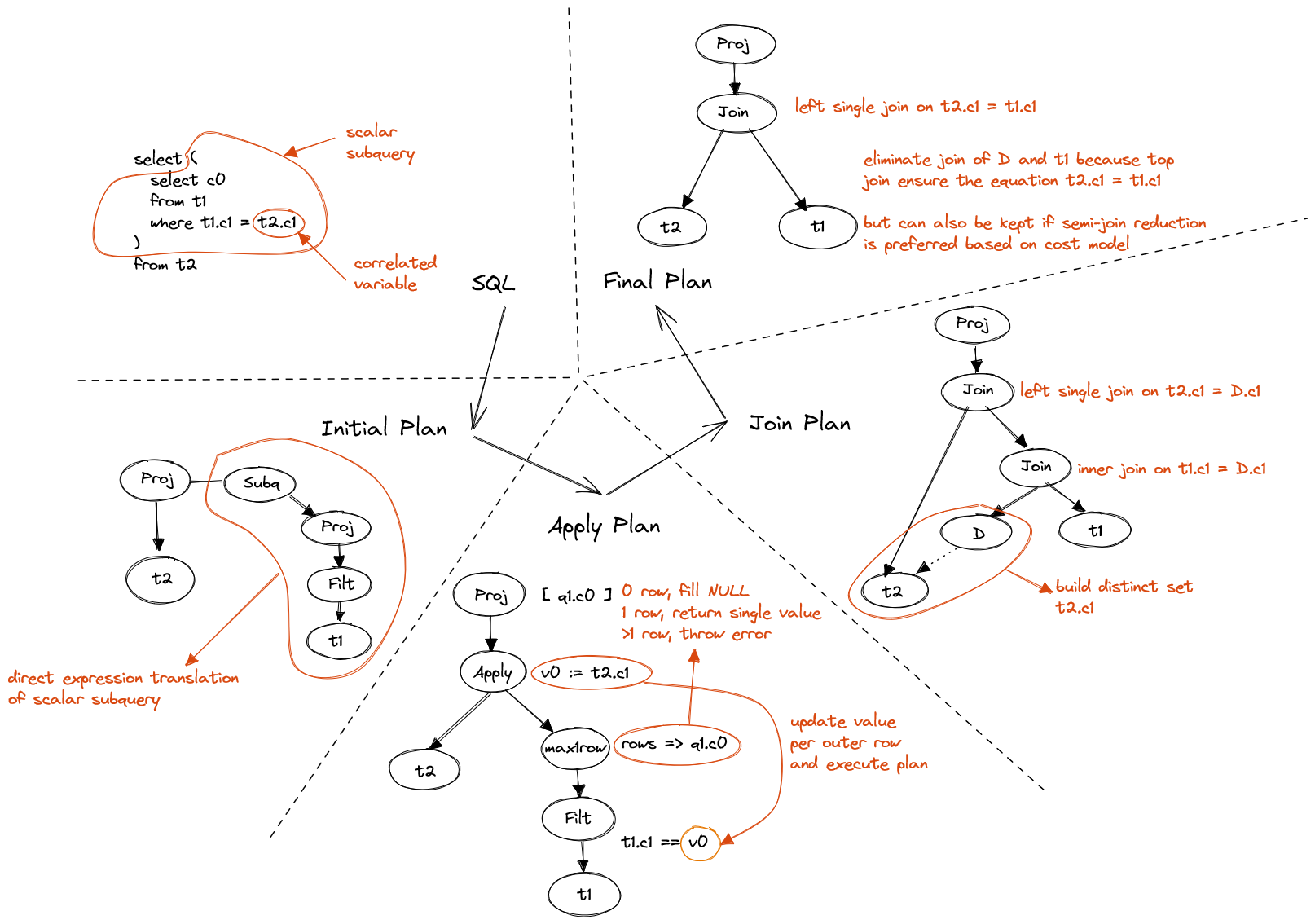

Figure 3. Correlated scalar subquery

The transformation from apply plan to join plan is non-trivial.

The basic idea is to create a distinct set of all correlated columns in middle.

on right side, it eliminates redundent computation. Assume we have 100 rows in t1 with identical c0, in apply plan, the right side will be executed 100 times, which is obviously a waste.

on left side, a simple left join can be performed to map results to original rows.

The transformation from join plan to final plan requires equality predicate of the correlated column t2.c1 to enable replacing t2.c1 with calculation on columns in t1.

Predicate	Eliminate D	Reason
t1.c1 = t2.c1	Y	trivial
t1.c1 = t2.c1 + 1	Y	convert to t2.c1 = t1.c1 - 1
t1.c1 = t1.c2 + t2.c1	Y	convert to t2.c1 = t1.c1 - t1.c2
t1.c1 = substring(t2.c1, 1, 2)	N	can not convert, but if we add Project before Join, we can
t1.c1 = t2.c1 and t1.c2 > t2.c2	N	can not convert, but if we remove second predicate, we can, we also need to add the removed condition to LeftSingleJoin later

This optimization is very similar to reversion of semi-join reduction. Suppose t1 is a remote table, t2 has very small NDV(Number of distinct values) on t2.c1, then table D is preferred to be generated and sent to remote to filter t1.

After all, we simplify the plan as final plan if possible, and keep the potential to convert it back to join plan in later optimization stage.

Non-correlated table subquery

EXISTS/NOT EXISTS

Non-correlated EXISTS and NOT EXISTS are converted to semi-join or anti-join with no join condition.

A limit operator could be added and pushed down to reduce data transfer.

SELECT c0 FROM t1
WHERE EXISTS (SELECT * FROM t2 WHERE c2 = 0)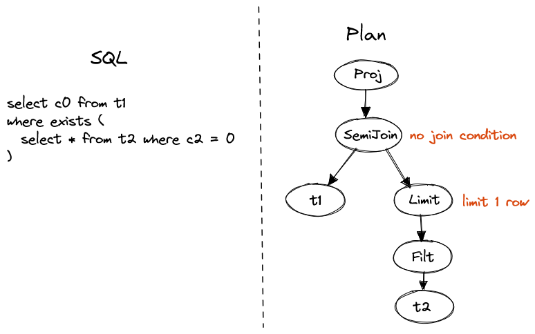

Figure 4. Non-correlated EXISTS

IN/NOT IN

The conversion of IN and NOT IN is non-trivial, because of three-value logic in SQL.

Three-value logic

The boolean expression in SQL has three values: true, false, null. The evaluation rule is as below.

Logical AND

left \ right	true	false	null
true	true	false	null
false	false	false	false
null	null	false	null

Logical OR

left \ right	true	false	null
true	true	true	true
false	true	false	null
null	true	null	null

Non-correlated IN can be converted to semi join if returned NULL can be treated as false, e.g. predicate with negative marker, or NULL value is forbidden, e.g. both sides have NOT NULL constraints.

Similarly, non-correlated NOT IN can be converted to anti join if returned NULL can be treated as true, e.g. predicate with positive marker, or NULL value is forbidden.

Positive/Negative marker of predicate

If returned null can be treated as false and do not impact the final result, the predicate is marked as negative. Otherwise, marked as positive.

To generate the marker, initialize with negative marker, once a NOT operator encountered, flip it.

WHERE c0 > 0; -- `c0 > 0` negative
WHERE NOT (c0 > 0 AND c1 > 0); -- `c0 > 0` positive, `c1 > 0` positive
WHERE NOT (c0 > 0 OR c1 > 0); -- same as above
WHERE NOT (c0 > 0 AND NOT c1 > 0); -- `c0 > 0` positive, `c1 > 0` negative

Otherwise, a left mark join should be generated, e.g. in projection.

Left semi join

Left semi join is similar to semi join, but it will retain all rows from left table, and append a match flag to each row. it's NULL free because all nulls involved in matching will be marked as false.

Left mark join

Left mark join is similar to left semi join, but it handles null values in specific columns and mark as null in matching instead of false.

SELECT c0 IN (SELECT c0 from t2) FROM t1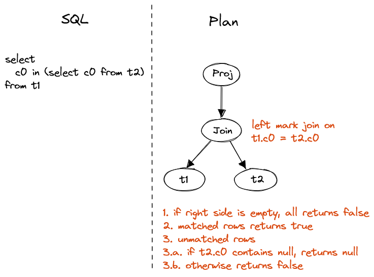

Figure 5. Non-correlated IN in projection

Special handling on NULL value and empty set is necessary, consider below cases:

1. 1 in () returns false. () means empty set, which is not valid SQL but can be generated by subquery.
2. null in () returns false. This is special because input is null and output is not null.
3. 1 in (1,2) returns true.
4. 1 in (2,3) returns false.
5. 1 in (1, null) returns true.
6. 1 in (2, null) returns null.

Quantified comparison

IN and NOT IN are special cases of quantified comparison. To handle non-equi quantified comparison, converting to semi join is not a good choice. Instead, we can aggregate the scalar result of inner subquery, cross apply to each row and evaluate corresponding expression.

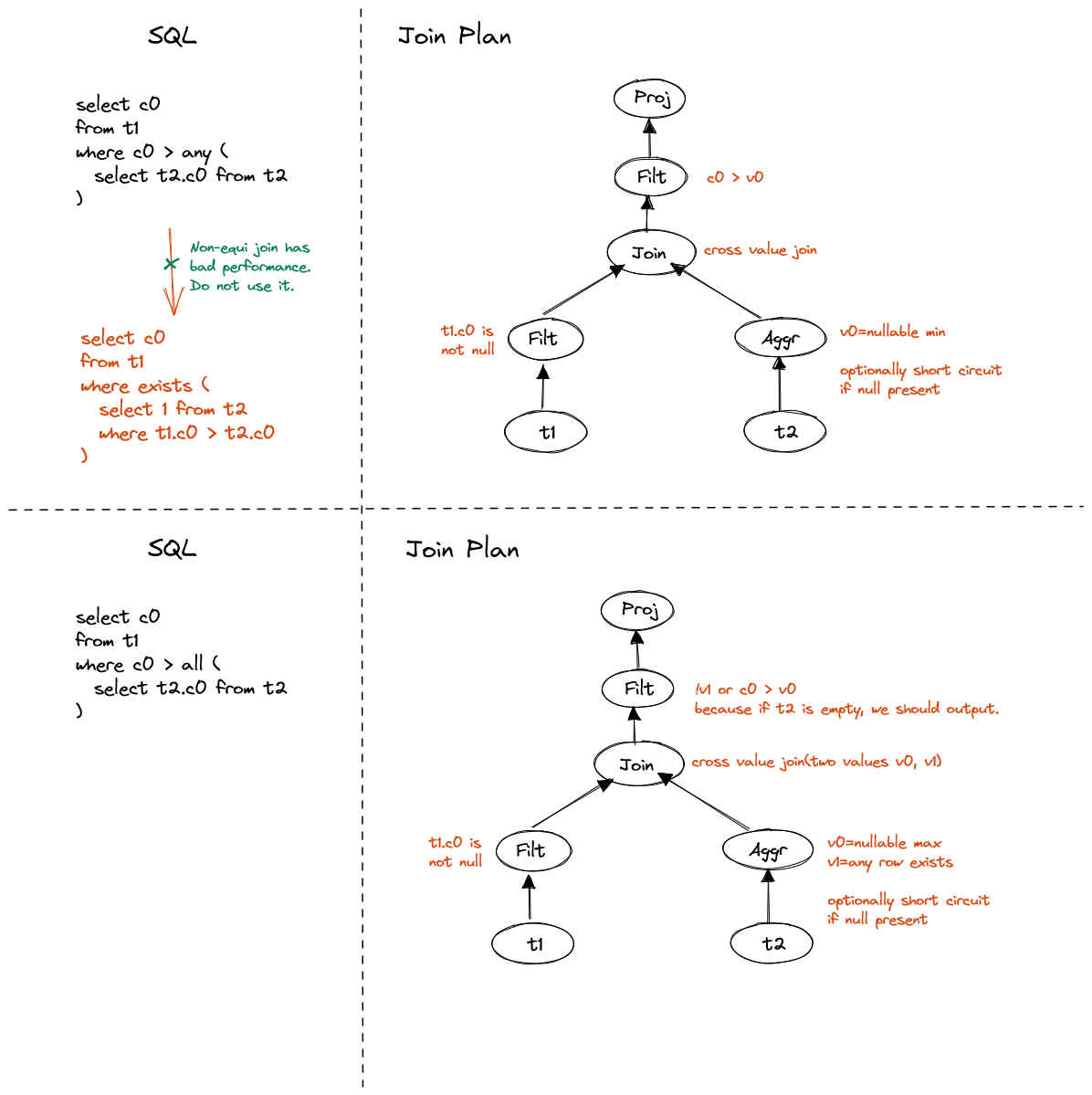
Figure 6. Non-correlated quantified comparison

Note: the cmp ALL case requires extra handling if the result set is empty. The expression is always true if inner data is empty.

Correlated table subquery

EXISTS/NOT EXISTS

It is trivial to convert EXISTS, NOT EXISTS to semi join, anti join, left semi join or left anti join.

IN/NOT IN

It's trivial to convert correlated IN to semi-join, in WHERE clause.

It's not trivial to convert correlated NOT IN, even in WHERE clause, because

1. Comparison between NULL and any value returns NULL.
2. NOT IN an empty list returns true, no matter what value is on left side, e.g NULL.
3. if a list contains NULL, even if the value on left side does not equal to any non-null values in the list, the result is still NULL.

SELECT c0 FROM t1
WHERE c0 NOT IN (
    SELECT t2.c0 FROM t2
    WHERE t1.c1 = t2.c1
)

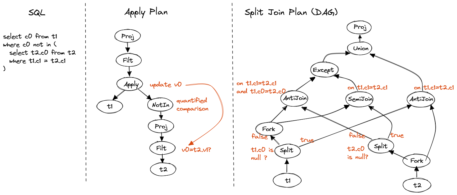
Figure 7. Correlated NOT IN

Between apply plan and split join plan(DAG) there could be anti join plan, which performs a anti join between t1 and t2. I skipped it because its core is still per-row execution, due to required special handling mentioned in non-correlated IN/NOT section.

To enable set-based execution, we have to switch operator tree to DAG(Directed Acyclic Graph), which supports fork and split operators on single node to feed multiple downstreams. The principle is to split data into multiple disjoint parts, process each part with simpler logic and merge them at the end.

Fork operator

Fork operator clones the input stream and provides two identical output streams.

Split operator

Split operator splits the input stream by given predicates and provides two identical output streams, matched and unmatched.

In this plan, we first split t1 into two parts based on nullable of t1.c0. The null part can anti join t2 without additional check, to output result in case of null in (). The non-null part will be cloned and join with splits of t2. As t1.c0 and t2.c0 are both non-null, a direct anti join can be performed. But the result is wrong as nulls in t2 is filtered, so we perform semi join on non-nulls in t1 to nulls in t2 and remove them from result of anti join. Finally union results of null part and non-null part of t1.

Quantified comparison

Correlated quantified comparision is a bit complex. The direct way to unnest such subquery may not be very beneficial, because adding non-equi join condition may not speed up the processing.

Instead, we should take serious consideration of the ordering property that comparison brings, e.g. > ANY means greater than at least one element, which could be translated to > MIN(values), and > ALL can be translated to > MAX(values).

Always take care of NULL and empty set if that impact the final result.

First, let's see projection.

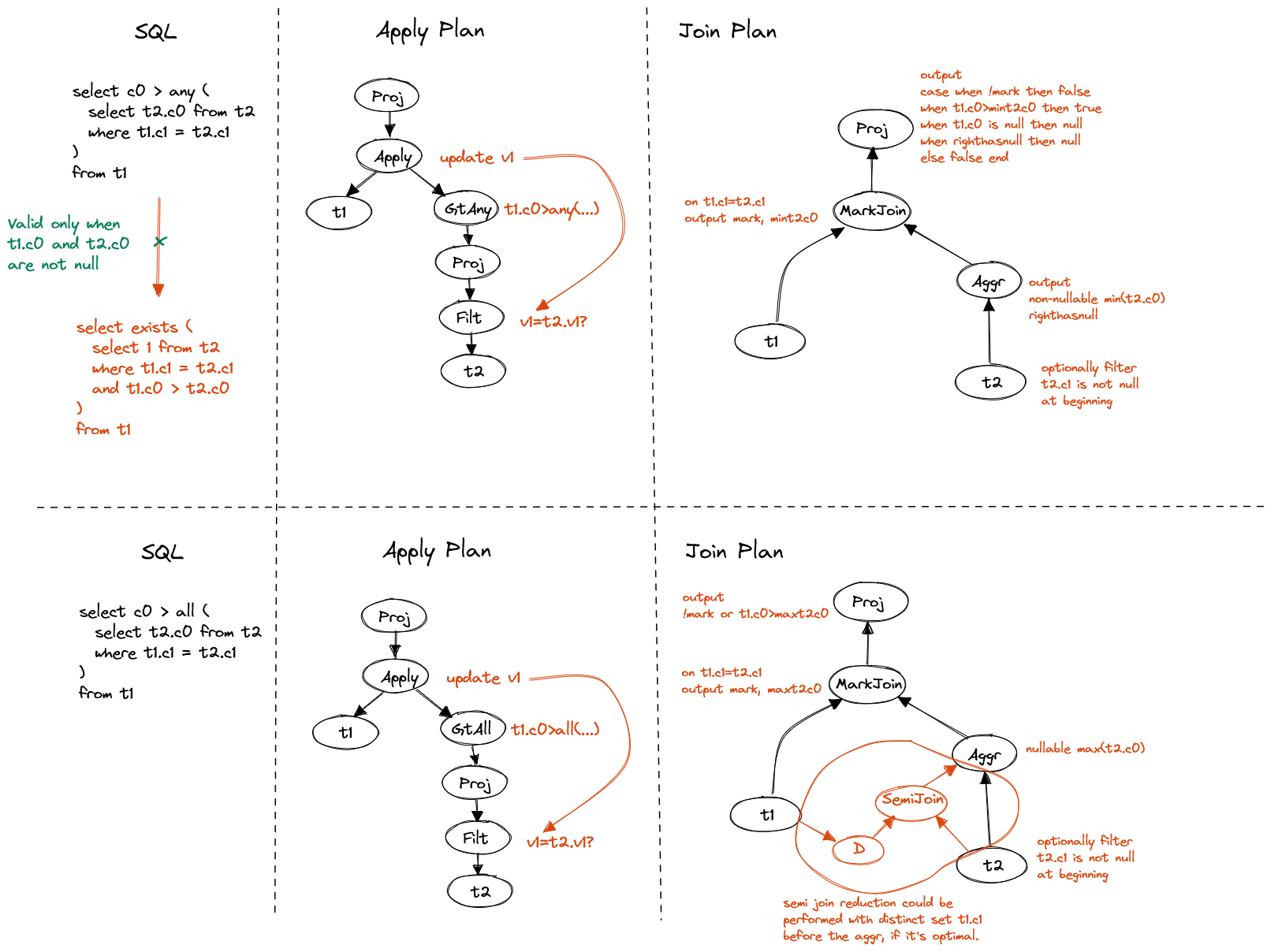
Figure 8. Correlated quantified comparison in projection

The conversion from quantified comparison to EXISTS is not available due to extra requirement on NULL handling. We can use mark join to propagate necessary attributes to evaluate the comparison. Additionally, semi-join reduction is free to perform before the aggregation, if cost model shows it's optimal.

Now, let's see filter.

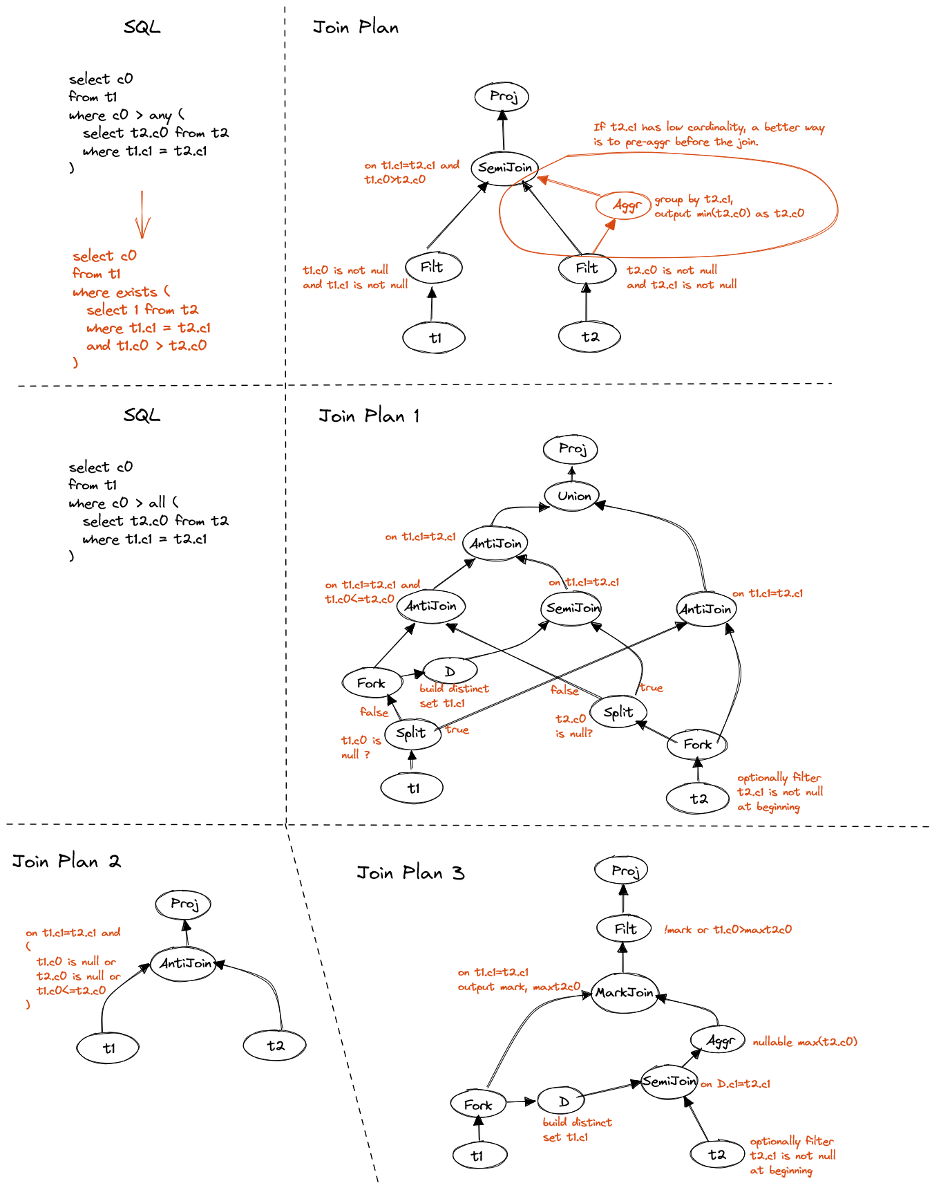
Figure 9. Correlated quantified comparison in filter

The ANY comparison can be directly translated to EXISTS subquery in WHERE clause, and then converted to semi join. Pretty simple, but if the equal join column has low cardinality, we may want to pre-aggregate before the join.

Disjunctive subquery

Below we talk about disjunctive subqueries. The main impact is that we have to build our plans as DAGs to fit for the disjunctive data processing.

Simple disjunction

SELECT c0 FROM t1
WHERE c1 > 100
OR EXISTS (
    SELECT * FROM t2
    WHERE t2.c1 = t1.c1
)

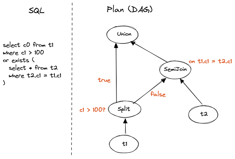
Figure 10. Disjunctive EXISTS

This is the simplest case of disjuctive subquery. We first caclulate c1 > 100, split data according to true/false flag(null treated as false). The false part is feed to semi join operator and join to t2. Finally union the true part and result of semi join.

If in disjunctive predicate the subquery precedes the comparison, we can swap them to end with same plan, as the join cost is often higher than filter cost. But in general the decision should be made by optimizer, based on the selectivity of each predicate.

And in more complex cases, the swap may not simplify the evaluation, for example the disjunction is composite of multiple subqueries, which we will talk about in next section.

Disjunctive outer predicate

SELECT c0 from t1
WHERE EXISTS (SELECT 1 FROM t2 WHERE t1.c1 = t2.c1)
OR NOT EXISTS (SELECT 1 FROM t3 WHERE t1.c2 = t3.c2)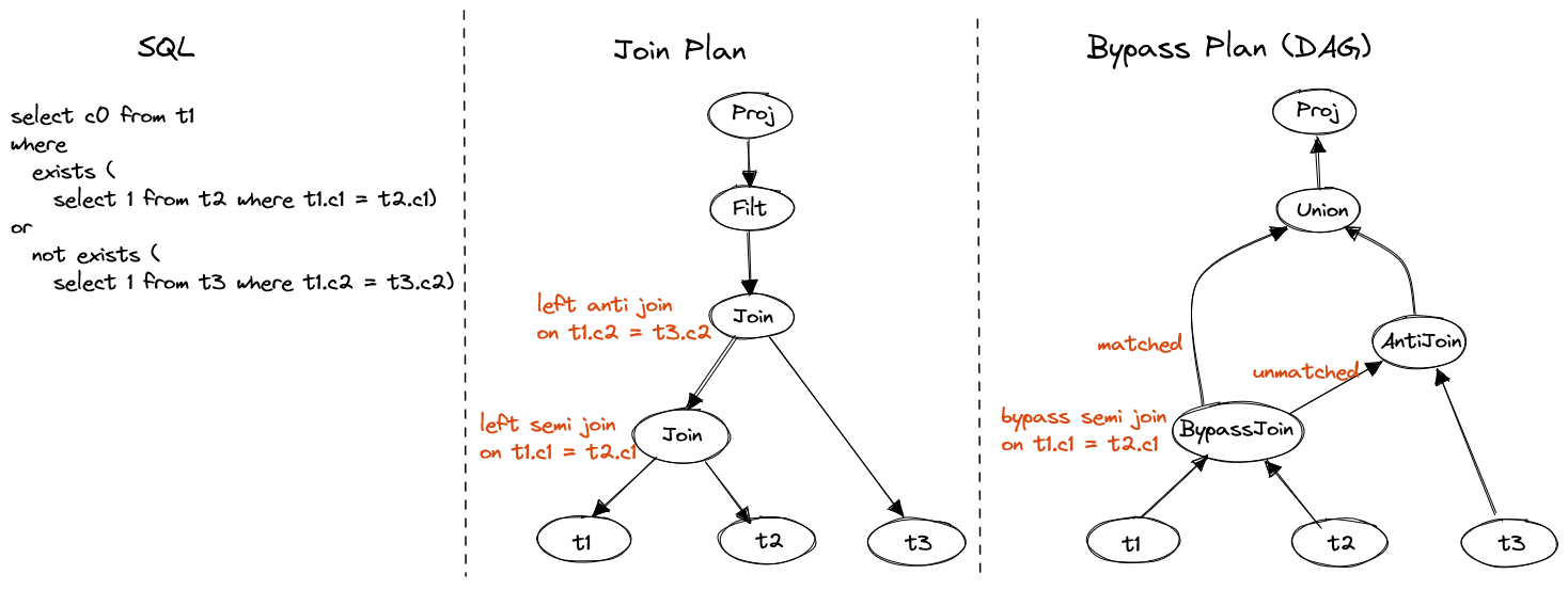

Figure 11. EXISTS or NOT EXISTS

There are two strategies to evaluate the query:

1. Keep the filter and use chained left joins to project all attributes required to evaluate the predicate.
2. Use bypass join to pipe the unmatched data to anti join and merge the matched data back.

The second strategy is better because only the necessary data is processed via disjunctive evaluation, but it requires DAG and introduces a new operator bypass join.

Bypass join

Different from common join operator, bypass join creates two output streams, one is for matched data, the other is for unmatched data. The unmatched data can be piped to next operator. It is the key operator to evaluate joins with disjunctive normal form.

Disjunctive inner predicate

SELECT (
    SELECT sum(c0) FROM t2
    WHERE t1.c1 = t2.c1 OR t1.c2 = t2.c2
)
FROM t1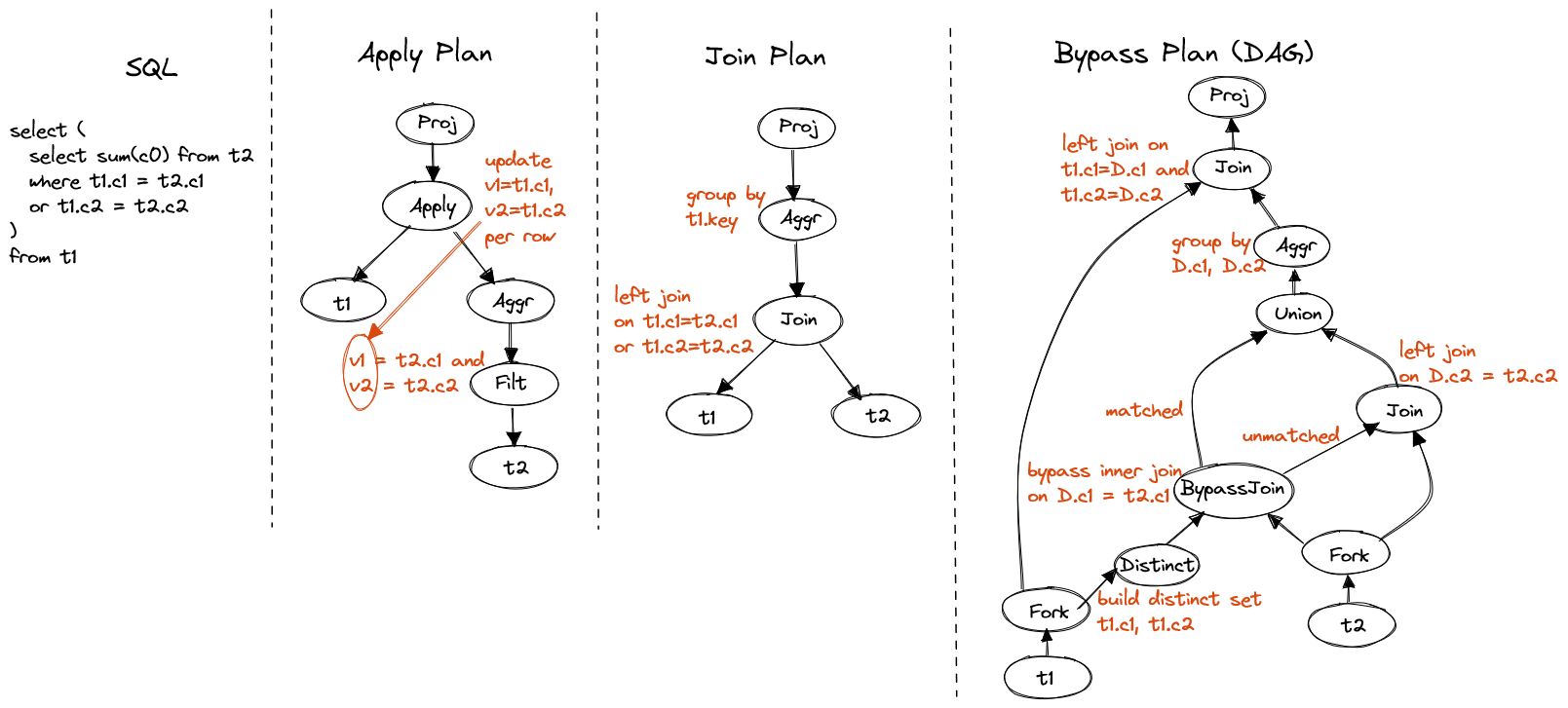

Figure 12. Disjunctive inner predicate

There are three strategies of disjunctive predicate inside subquery, which is very similar to join condition, and can be applied to evaluate disjunctive joins.

1. Use apply operator to evaluate the aggregation per row of t1.
2. Convert apply to left join. This will not gain performance as the disjunctive join condition prevent optimizer to choose an efficient join algorithm like hash join or merge join.
3. First generate a distinct set holding key, c1 and c2 int1. Use bypass join to select rows that match first predicate and pipe the unmatched rows to left join. Then union and aggregate result sets of both joins. Finally join back to t1 on its key.

The generated plan of the 3rd strategy looks complicated, but it's actually very efficient. First if t1 has low cardinality on c1 and c2, the distinct set will largely reduce redundent computation. Second, both bypass join and left join can be implemented using efficient hash algorithm.

In addition, the optimizer is able to generate another plan that eliminates the distinct set at bottom and join on top, by keeping key of t1 in whole path. It is preferred if t1 has high cardinality.

Subquery of joins

Inner join

SELECT (
    SELECT sum(t2.c0 + t3.c0) FROM t2, t3
    WHERE t2.c1 = t1.c1
    AND t3.c3 = 0
)
FROM t1

If correlated column only present in predicate with one table, join D with it and then join the other table.

SELECT (
    SELECT sum(t2.c0 + t3.c0) FROM t2, t3
    WHERE t2.c1 = t1.c1
    AND t3.c3 = t1.c0
)
FROM t1

If correlated column present in predicates with both tables, join D with both tables and then natural join back with additional euqal predicate of D's columns.

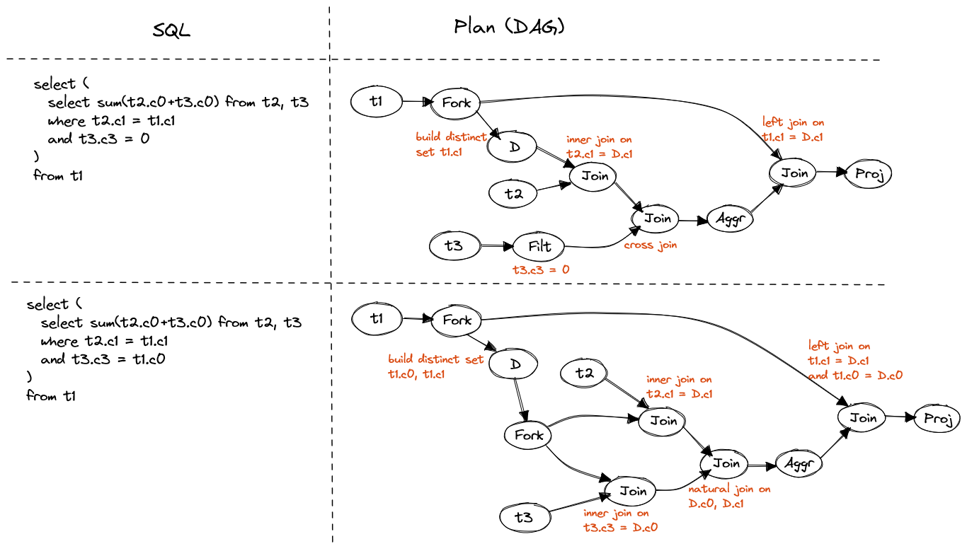
Figure 13. Inner join in subquery

Outer join

SELECT (
    SELECT sum(t2.c0) 
    FROM t2 LEFT JOIN t3
    ON t3.c3 = t1.c1
)
FROM t1

If correlated column present only in predicates with left table, join D with left table, then left join right table. Otherwise, join D with both tables and then left join back.

SELECT (
    SELECT sum(t2.c0) + sum(t3.c0) 
    FROM t2 FULL JOIN t3
    ON t2.c1 = t3.c1
    AND t2.c2 = t1.c1
    AND t3.c3 = t1.c1
)
FROM t1

Join D with both tables and then full join back.

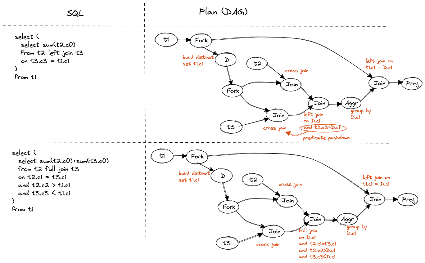
Figure 14. Outer join in subquery

The corss join looks very bad, but in actual use case, if the correlated is in WHERE clause, outer join can be converted to inner join and predicates can be pushed down to single table.

Nested Subquery

SELECT (
    SELECT SUM(c0) FROM t2
    WHERE t1.c1 = t2.c1
    AND t2.c0 > (
        SELECT SUM(c3) FROM t3
        WHERE t2.c2 = t3.c2
    )
)
FROM t1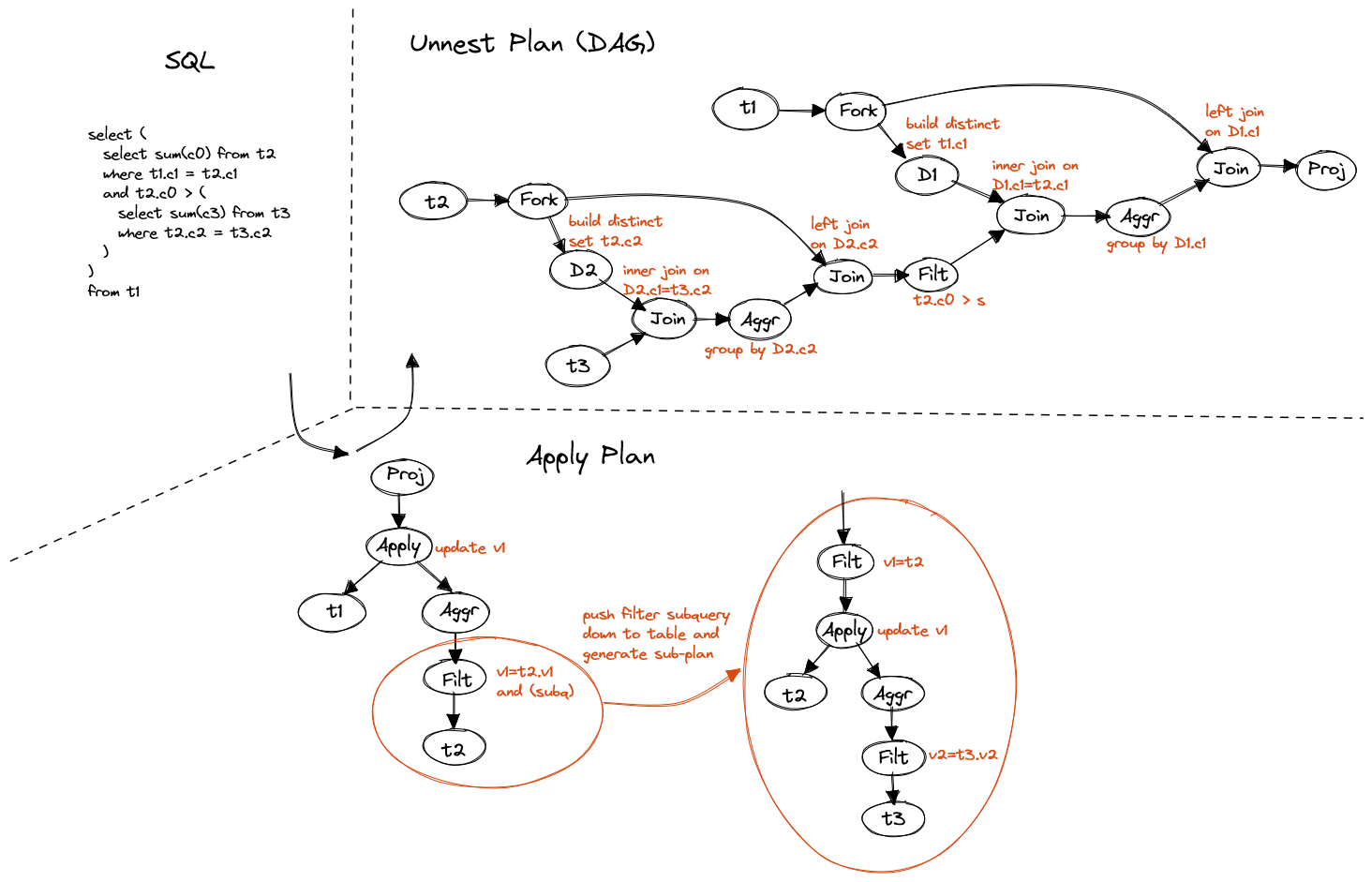

Figure 15. Chained nested subquery

Chained subquery can be resolved recursively. Inner subquery is identified and converted first, then outer one.

If correlated column does not belong to direct parent, e.g. in below query, t1.c2 refers to the outermost table, we can level it up, just like handling a non-correlated subquery, to solve it before entering current level.

SELECT (
    SELECT SUM(c0) FROM t2
    WHERE t1.c1 = t2.c1
    AND t2.c0 > (
        SELECT SUM(c3) FROM t3
        WHERE t1.c2 = t3.c2
    )
)
FROM t1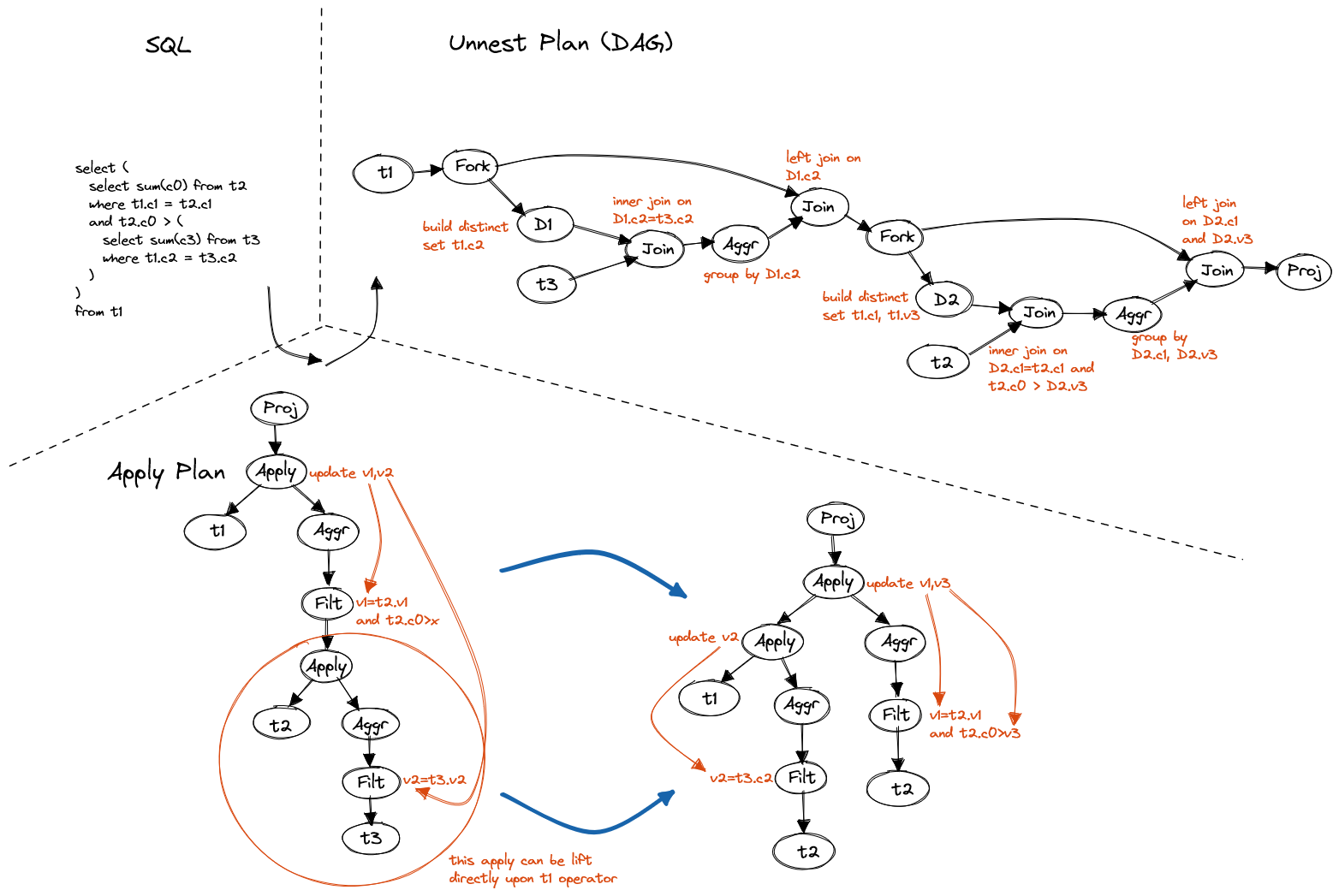

Figure 16. Lifting nested subquery

The most complicated nested subquery is the one that has correlated columns in different levels, e.g. like below the innermost subquery has two correlated columns, t2.c2 is from direct parent, t1.c2 is from grand-parent.

SELECT (
    SELECT SUM(c0) FROM t2
    WHERE t1.c1 = t2.c1
    AND t2.c0 > (
        SELECT SUM(c3) FROM t3
        WHERE t1.c2 = t3.c2
        AND t2.c2 = t3.c2
    )
)
FROM t1

We're still able to unnest it.

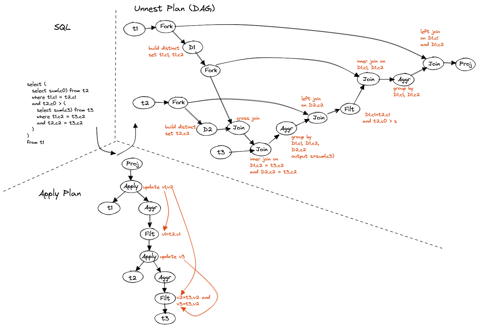
Figure 17. Cross-level nested subquery

Implementation

Operator

todo

Rule

todo

Optimization

todo

References

1. C. A. Galindo-Legaria, M. Joshi: Orthogonal Optimization of Subqueries and Aggregation.
2. M. Elhemali, C. A. Galindo-Legaria: Execution Strategies for SQL Subqueries.
3. T. Newmann, A. Kemper: Unnesting Arbitrary Queries.
4. M. Steinbrunn, K. Peithner: Bypassing Joins in Disjunctive Queries.
5. J. Claussen, A. Kemper: Optimization and Evaluation of Disjunctive Queries.
6. S. Bellamkonda, R. Ahmed: Enhanced Subquery Optimizations in Oracle.