ReactiveMP.jl

Documentation	Build Status	Coverage	Zenodo DOI	Pkg Eval

ReactiveMP.jl is a Julia package for automatic Bayesian inference on a factor graph with reactive message passing.

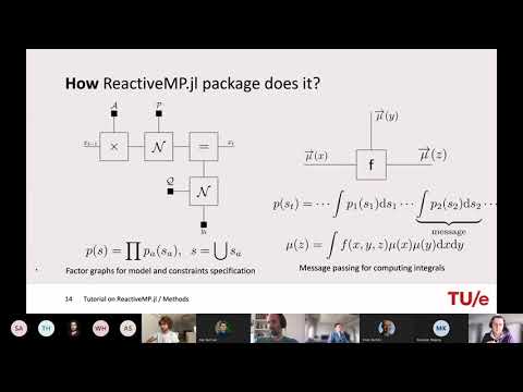
Given a probabilistic model, ReactiveMP allows for an efficient message-passing based Bayesian inference. It uses the model structure to generate an algorithm that consists of a sequence of local computations on a Forney-style factor graph (FFG) representation of the model.

The current version supports belief propagation (sum-product message passing) and variational message passing (both Mean-Field and Structured VMP) and is aimed to run inference in conjugate state-space models.

ReactiveMP.jl has been designed with a focus on efficiency, scalability and maximum performance for running inference on conjugate state-space models with message passing. Below is a benchmark comparison between ReactiveMP.jl and Turing.jl on a linear multivariate Gaussian state space Model. It is worth noting that this model contains many conjugate prior and likelihood pairings that lead to analytically computable Bayesian posteriors. For these types of models, ReactiveMP.jl takes advantage of the conjugate pairings and beats general-purpose probabilistic programming packages easily in terms of computational load, speed, memory and accuracy. On the other hand, sampling-based packages like Turing.jl are generic Bayesian inference solutions and are capable of running inference for a broader set of models.

Code is available in benchmark folder:

Turing comparison	Scalability performance

Overview

See the videos below from JuliaCon 2021 and BIASlab seminar for a quick introduction to ReactiveMP.

JuliaCon 2021 presentation	ReactiveMP.jl API tutorial

Installation

Install ReactiveMP through the Julia package manager:

] add ReactiveMP

Optionally, use ] test ReactiveMP to validate the installation by running the test suite.

Getting Started

There are demos available to get you started in the demo/ folder. Comparative benchmarks are available in the benchmarks/ folder.

Coin flip simulation

Here we show a simple example of how to use ReactiveMP.jl for Bayesian inference problems. In this example we want to estimate a bias of a coin in a form of a probability distribution in a coin flip simulation.

Let's start by creating some dataset. For simplicity in this example we will use static pre-generated dataset. Each sample can be thought of as the outcome of single flip which is either heads or tails (1 or 0). We will assume that our virtual coin is biased, and lands heads up on 75% of the trials (on average).

First let's setup our environment by importing all needed packages:

using Rocket, GraphPPL, ReactiveMP, Distributions, Random

Next, let's define our dataset:

n = 500  # Number of coin flips
p = 0.75 # Bias of a coin

distribution = Bernoulli(p) 
dataset      = float.(rand(Bernoulli(p), n))

Model specification

In a Bayesian setting, the next step is to specify our probabilistic model. This amounts to specifying the joint probability of the random variables of the system.

Likelihood

We will assume that the outcome of each coin flip is governed by the Bernoulli distribution, i.e.

where represents "heads", represents "tails". The underlying probability of the coin landing heads up for a single coin flip is .

Prior

We will choose the conjugate prior of the Bernoulli likelihood function defined above, namely the beta distribution, i.e.

where a and b are the hyperparameters that encode our prior beliefs about the possible values of θ. We will assign values to the hyperparameters in a later step.

Joint probability

The joint probability is given by the multiplication of the likelihood and the prior, i.e.

Now let's see how to specify this model using GraphPPL's package syntax.

# GraphPPL.jl export `@model` macro for model specification
# It accepts a regular Julia function and builds an FFG under the hood
@model function coin_model(n)

    # `datavar` creates data 'inputs' in our model
    # We will pass data later on to these inputs
    # In this example we create a sequence of inputs that accepts Float64
    y = datavar(Float64, n)
    
    # We endow θ parameter of our model with some prior
    θ ~ Beta(2.0, 7.0)
    
    # We assume that outcome of each coin flip 
    # is governed by the Bernoulli distribution
    for i in 1:n
        y[i] ~ Bernoulli(θ)
    end
    
    # We return references to our data inputs and θ parameter
    # We will use these references later on during inference step
    return y, θ
end

As you can see, GraphPPL offers a model specification syntax that resembles closely to the mathematical equations defined above. We use datavar function to create "clamped" variables that take specific values at a later date. θ ~ Beta(2.0, 7.0) expression creates random variable θ and assigns it as an output of Beta node in the corresponding FFG.

Inference specification

Once we have defined our model, the next step is to use ReactiveMP API to infer quantities of interests. To do this we can use a generic inference function from ReactiveMP.jl that supports static datasets.

result = inference(
    model = Model(coin_model, length(data)),
    data  = (y = data, )
)

There is a way to manually specify an inference procedure for advanced use-cases. ReactiveMP API is flexible in terms of inference specification and is compatible both with real-time inference processing and with static datasets. In most of the cases for static datasets, as in our example, it consists of same basic building blocks:

1. Return variables of interests from model specification
2. Subscribe on variables of interests posterior marginal updates
3. Pass data to the model
4. Unsubscribe

Here is an example of inference procedure:

function custom_inference(data)
    n = length(data)

    # `coin_model` function from `@model` macro returns a reference to 
    # the model object and the same output as in `return` statement 
    # in the original function specification
    model, (y, θ) = coin_model(n)
    
    # Reference for future posterior marginal 
    mθ = nothing

    # `getmarginal` function returns an observable of 
    # future posterior marginal updates
    # We use `Rocket.jl` API to subscribe on this observable
    # As soon as posterior marginal update is available we just save it in `mθ`
    subscription = subscribe!(getmarginal(θ), (m) -> mθ = m)
    
    # `update!` function passes data to our data inputs
    update!(y, data)
    
    # It is always a good practice to unsubscribe and to 
    # free computer resources held by the subscription
    unsubscribe!(subscription)
    
    # Here we return our resulting posterior marginal
    return mθ
end

Inference execution

Here after everything is ready we just call our inference function to get a posterior marginal distribution over θ parameter in the model.

θestimated = custom_inference(dataset)

Where to go next?

There are a set of demos available in ReactiveMP repository that demonstrate the more advanced features of the package. Alternatively, you can head to the documentation that provides more detailed information of how to use ReactiveMP and GraphPPL to specify probabilistic models.

License

MIT License Copyright (c) 2021-2022 BIASlab