


AstroLink is a general purpose clustering algorithm built for extracting meaningful hierarchical structure from astrophysical data sets. In practice AstroLink rarely requires any parameter tuning before application, nevertheless, it has a small number intuitive-to-adjust parameters should this be necessary. As such, it is readily capable of finding an arbitary number of arbitrarily shaped clusters (and their structural relationship within the broader hierarchy) from arbitrarily defined data sets. Clusters found by AstroLink are defined as being statistically distinct overdensities when compared to their surrounds and to the noisy density fluctuations within the data set.
The AstroLink documentation can be found on ReadTheDocs. The original AstroLink science paper also provides further detailed information.
The Python package astrolink can be installed from PyPI:
python -m pip install astrolink
Or, if you use Anaconda:
conda install -c conda-forge astrolink
AstroLink can be easily applied to any point-based input data expressed as a np.ndarray with shape (n_samples, d_features).
So first we need some data...
import numpy as np
import sklearn.datasets as data

# Generate some structured data with noise
np.random.seed(0)
background = np.random.uniform(-2, 2, (1000, 2))
moons, _ = data.make_moons(n_samples = 2000, noise = 0.1)
moons -= np.array([[0.5, 0.25]])    # centres moons on origin
gauss_1 = np.random.normal(-1.25, 0.2, (500, 2))
gauss_2 = np.random.normal(1.25, 0.2, (500, 2))

P = np.vstack([background, moons, gauss_1, gauss_2])
... then we run AstroLink over that data...
from astrolink import AstroLink

clusterer = AstroLink(P)
clusterer.run()
... and that's it, AstroLink has found the hierarchical clustering structure of P!
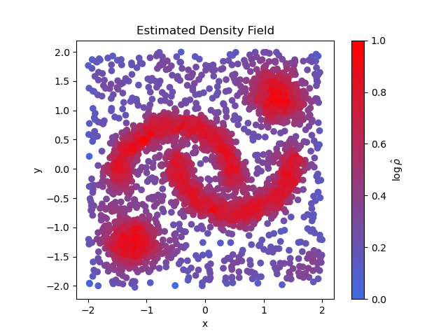
For low-dimensional input data, like we have in this example, it is then possible to visualise the estimated density field by plotting the input data and colouring it by the logRho attribute.
import matplotlib.pyplot as plt
from matplotlib.colors import LinearSegmentedColormap as lscm

# Colour map that shows low/high values in blue/red
cm = lscm.from_list('density', [(0, 'royalblue'), (1, 'red')])

# Plot the data with colorbar
fig, ax = plt.subplots()
d_field = ax.scatter(P[:, 0], P[:, 1], c = clusterer.logRho, cmap = cm)
plt.colorbar(d_field, label = r'$\log\hat\rho$', ax = ax)

# Tidy up
ax.set_title('Estimated Density Field')
ax.set_xlabel('x')
ax.set_ylabel('y')
ax.set_aspect('equal')

# Show plot
plt.show()
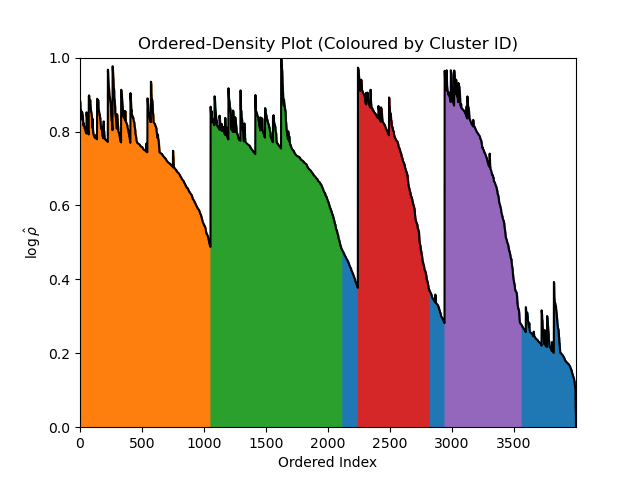
Regardless of the dimensionality of the input data, the clustering structure within it can always be visualised via the 2-dimensional AstroLink ordered-density plot.
# Plot the data
fig, ax = plt.subplots()
ax.plot(range(clusterer.n_samples), clusterer.logRho[clusterer.ordering])

# Tidy up
ax.set_xlim(0, clusterer.n_samples - 1)
ax.set_ylim(0, 1)
ax.set_title('Ordered-Density Plot')
ax.set_xlabel('Ordered Index')
ax.set_ylabel(r'$\log\hat\rho$')

# Show plot
plt.show()

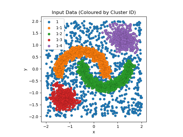
Although, since the input data in this example can be easily visualised as well, we may as well view this alongside the clusters themselves (as predicted by AstroLink).
# Create two figures
fig1, ax1 = plt.subplots()
fig2, ax2 = plt.subplots()

# Make the ordered-density plot
ax1.plot(range(clusterer.n_samples), clusterer.logRho[clusterer.ordering], c = 'k', zorder = 2)

# Colour the ordered-density and input data plots by each cluster
for i, (clst, clst_id) in enumerate(zip(clusterer.clusters, clusterer.ids)):
    # Indices of points in cluster
    clst_members = clusterer.ordering[clst[0]:clst[1]]

    # Section of ordered-density plot corresponding to cluster
    clst_ordered_density = clusterer.logRho[clst_members]
    ax1.fill_between(range(clst[0], clst[1]), clst_ordered_density, color = f"C{i}", zorder = 1)

    # Points in cluster
    clst_P = P[clst_members]
    ax2.scatter(clst_P[:, 0], clst_P[:, 1], facecolors = f"C{i}", edgecolors = 'k', lw = 0.1, label = clst_id)

# Tidy up
ax1.set_xlim(0, clusterer.n_samples - 1)
ax1.set_ylim(0, 1)
ax1.set_title('Ordered-Density Plot (Coloured by Cluster ID)')
ax1.set_xlabel('Ordered Index')
ax1.set_ylabel(r'$\log\hat\rho$')
ax2.set_title('Input Data (Coloured by Cluster ID)')
ax2.set_xlabel('x')
ax2.set_ylabel('y')
ax2.set_aspect('equal')
ax2.legend(framealpha = 1)

# Show plot
plt.show()
Note
AstroLink always returns a cluster that is equal to the entire input data (with ID '1' by default) which allows it to be (re-)applied to a disjoint data set in a modular fashion.
To do further analysis on the clustering output, the user may wish to know which points (with respect to the order in which they appear within the input data) belong to the clusters that AstroLink has found. These sets can be constructed from the ordering and clusters attributes.
cluster_members = [clusterer.ordering[clst[0]:clst[1]] for clst in clusterer.clusters]
If you want to contribute to the development of astrolink, we recommend
the following editable installation from this repository:
git clone https://github.com/william-h-oliver/astrolink.git
cd astrolink
python -m pip install --editable .[tests]
Having done so, the test suite can then be run using pytest:
python -m pytest
If you have used AstroLink in a scientific publication, please use the following citation:
@ARTICLE{Oliver2024,
       author = {{Oliver}, William H. and {Elahi}, Pascal J. and {Lewis}, Geraint F. and {Buck}, Tobias},
        title = "{The hierarchical structure of galactic haloes: differentiating clusters from stochastic clumping with ASTROLINK}",
      journal = {\mnras},
     keywords = {methods: data analysis, methods: statistical, galaxies: star clusters: general, galaxies: structure, Astrophysics - Astrophysics of Galaxies},
         year = 2024,
        month = may,
       volume = {530},
       number = {3},
        pages = {2637-2647},
          doi = {10.1093/mnras/stae1029},
archivePrefix = {arXiv},
       eprint = {2312.14632},
 primaryClass = {astro-ph.GA},
       adsurl = {https://ui.adsabs.harvard.edu/abs/2024MNRAS.530.2637O},
      adsnote = {Provided by the SAO/NASA Astrophysics Data System}
}
This repository was set up using the SSC Cookiecutter for Python Packages.